0.引言

• PL-VIO，本文关注线段。
• 论文链接
• SLAM中线特征的参数化和求导
• SLAM线特征学习（1）——基本的线特征表示与优化推导
• SLAM线特征学习（2）——线特征初始化和最小表示
• SLAM中线特征的参数化表示方法/重投影/初始化方法

1.LineFeatureTracker核心逻辑解读

• 数据结构定义：

struct Line {Point2f StartPt;Point2f EndPt;float lineWidth;Point2f Vp;Point2f Center;Point2f unitDir;  // [cos(theta), sin(theta)]float length;float theta;// para_a * x + para_b * y + c = 0float para_a;float para_b;float para_c;float image_dx;float image_dy;float line_grad_avg;float xMin;float xMax;float yMin;float yMax;unsigned short id;int colorIdx;
};class FrameLines {public:int frame_id;Mat img;vector<Line> vecLine;vector<int> lineID;// opencv3 lsd+lbdstd::vector<KeyLine> keylsd;Mat lbd_descr;
};

• keylsd：提取的线段结果（经过长度筛选的，太短的不要）
• keylbd_descr：对应线段描述子结果（经过长度筛选的，太短的不要）
• 新进的img提取线特征：
  • 如果是第一帧img：forwframe_->lineID.push_back(allfeature_cnt++)；（allfeature_cnt是整个系统全局的线特征计数）,因此lineID是全局的ID，整个系统中线特征具有唯一的ID。update:后面更新的是没匹配上的。
  • 如果不是第一帧img，则暂时赋值为-1，但forwframe_->lineID数组的size的大小是和keylsd相同的；
    • 匹配后将-1进行更改：forwframe_->lineID[mt.queryIdx] = curframe_->lineID[mt.trainIdx];
      • Key = 当前帧线段的ID
      • Value = 前一帧线段的lineID[mt.trainIdx]
    • 判断当前帧水平，垂直方向线段数量是否分别足够35条，不够的补上。

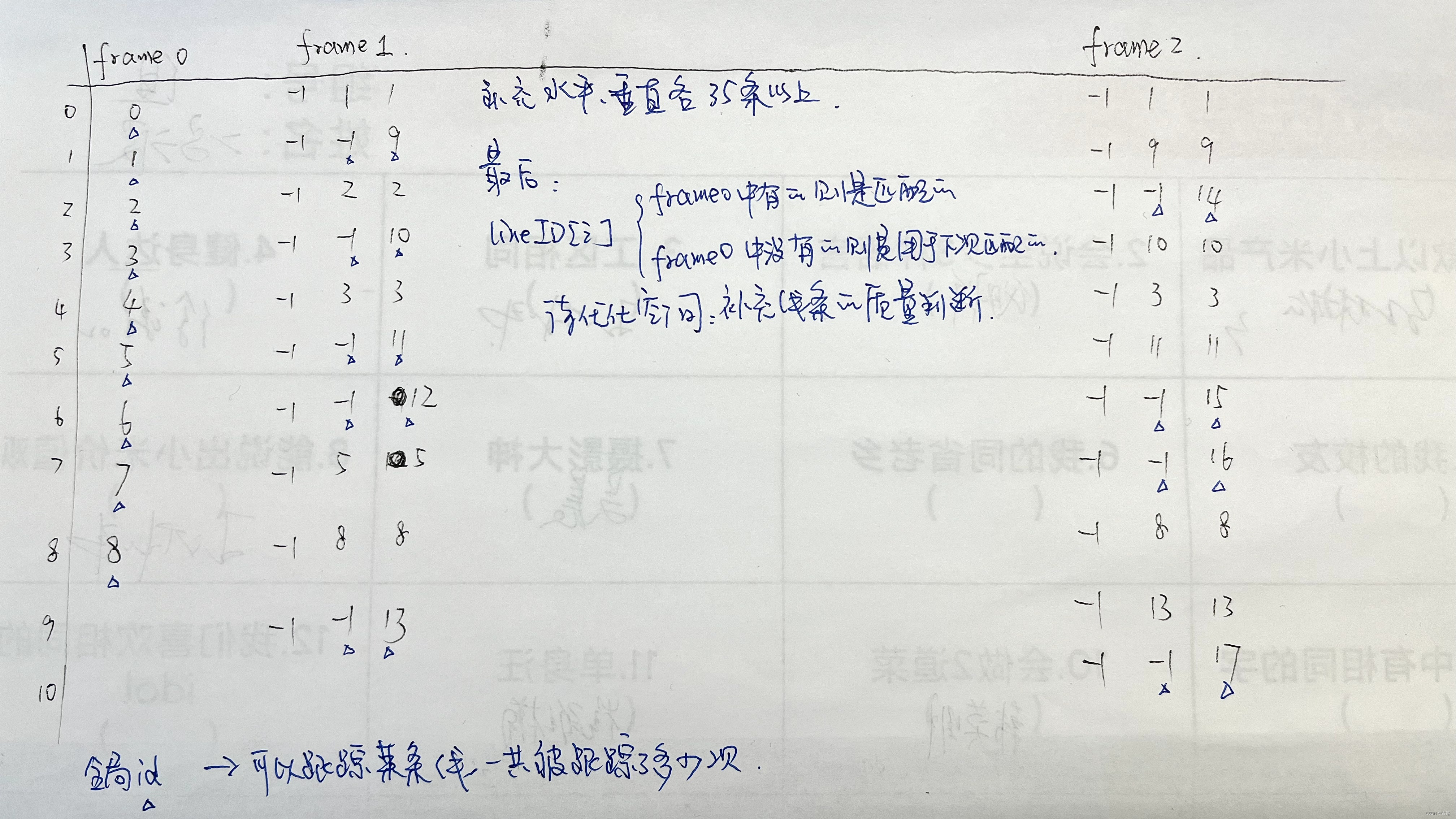
匹配的结果，对应关系，其实就是存储的全局ID信息。

代码注释，可惜另一个函数的关键内容lineDetector没放出来，这个函数的vecLine只在最后做了一个转换。frame_id没维护。

void LineFeatureTracker::readImage(const cv::Mat &_img) {cv::Mat img;TicToc t_p;frame_cnt++;//   cv::remap(_img, img, undist_map1_, undist_map2_, CV_INTER_LINEAR);cv::remap(_img, img, undist_map1_, undist_map2_, cv::INTER_LINEAR);//    cv::imshow("lineimg",img);//    cv::waitKey(1);// ROS_INFO("undistortImage costs: %fms", t_p.toc());if (EQUALIZE)  // 直方图均衡化{cv::Ptr<cv::CLAHE> clahe = cv::createCLAHE(3.0, cv::Size(8, 8));clahe->apply(img, img);}bool first_img = false;if (forwframe_ == nullptr)  // 系统初始化的第一帧图像{forwframe_.reset(new FrameLines);curframe_.reset(new FrameLines);forwframe_->img = img;curframe_->img = img;  // 上一帧first_img = true;} else {forwframe_.reset(new FrameLines);  // 初始化一个新的帧forwframe_->img = img;             // 当前帧}TicToc t_li;Ptr<line_descriptor::LSDDetectorC> lsd_ =line_descriptor::LSDDetectorC::createLSDDetectorC();// lsd parametersline_descriptor::LSDDetectorC::LSDOptions opts;opts.refine = 1;   // 1     	The way found lines will be refinedopts.scale = 0.5;  // 0.8   	The scale of the image that will be used to find// the lines. Range (0..1].opts.sigma_scale = 0.6;  // 0.6  	Sigma for Gaussian filter. It is// computed as sigma = _sigma_scale/_scale.opts.quant =2.0;  // 2.0   Bound to the quantization error on the gradient normopts.ang_th = 22.5;  // 22.5	Gradient angle tolerance in degreesopts.log_eps = 1.0;  // 0		Detection threshold: -log10(NFA) >// log_eps. Used only when advance refinement is chosenopts.density_th = 0.6;  // 0.7	Minimal density of aligned region points// in the enclosing rectangle.opts.n_bins =1024;  // 1024 	Number of bins in pseudo-ordering of gradient modulus.double min_line_length =0.125;  // Line segments shorter than that are rejected// opts.refine       = 1;// opts.scale        = 0.5;// opts.sigma_scale  = 0.6;// opts.quant        = 2.0;// opts.ang_th       = 22.5;// opts.log_eps      = 1.0;// opts.density_th   = 0.6;// opts.n_bins       = 1024;// double min_line_length = 0.125;opts.min_length = min_line_length * (std::min(img.cols, img.rows));std::vector<KeyLine> lsd, keylsd;// void LSDDetectorC::detect( const std::vector<Mat>& images,// std::vector<std::vector<KeyLine> >& keylines, int scale, int numOctaves,// const std::vector<Mat>& masks ) constlsd_->detect(img, lsd, 2, 1, opts);// visualize_line(img,lsd);// step 1: line extraction// TicToc t_li;// std::vector<KeyLine> lsd, keylsd;// Ptr<LSDDetector> lsd_;// lsd_ = cv::line_descriptor::LSDDetector::createLSDDetector();// lsd_->detect( img, lsd, 2, 2 );sum_time += t_li.toc();ROS_INFO("line detect costs: %fms", t_li.toc());Mat lbd_descr, keylbd_descr;// step 2: lbd descriptorTicToc t_lbd;Ptr<BinaryDescriptor> bd_ = BinaryDescriptor::createBinaryDescriptor();bd_->compute(img, lsd, lbd_descr);// std::cout<<"lbd_descr = "<<lbd_descr.size()<<std::endl;//for (int i = 0; i < (int)lsd.size(); i++) {if (lsd[i].octave == 0 && lsd[i].lineLength >= 60) {  // 对长度做一个筛选keylsd.push_back(lsd[i]);keylbd_descr.push_back(lbd_descr.row(i));}}// std::cout<<"lbd_descr = "<<lbd_descr.size()<<std::endl;//    ROS_INFO("lbd_descr detect costs: %fms", keylsd.size() * t_lbd.toc() ///    lsd.size() );sum_time += keylsd.size() * t_lbd.toc() / lsd.size();///forwframe_->keylsd = keylsd;  // 当前帧的关键线段forwframe_->lbd_descr = keylbd_descr;for (size_t i = 0; i < forwframe_->keylsd.size(); ++i) {if (first_img)forwframe_->lineID.push_back(allfeature_cnt++);elseforwframe_->lineID.push_back(-1);  // give a negative id}// if(!first_img)// {//     std::vector<DMatch> lsd_matches;//     Ptr<BinaryDescriptorMatcher> bdm_;//     bdm_ = BinaryDescriptorMatcher::createBinaryDescriptorMatcher();//     bdm_->match(forwframe_->lbd_descr, curframe_->lbd_descr, lsd_matches);//     visualize_line_match(forwframe_->img.clone(), curframe_->img.clone(),//     forwframe_->keylsd, curframe_->keylsd, lsd_matches);//     // std::cout<<"lsd_matches = "<<lsd_matches.size()<<"//     forwframe_->keylsd = "<<keylbd_descr.size()<<" curframe_->keylsd =//     "<<keylbd_descr.size()<<std::endl;// }if (curframe_->keylsd.size() > 0) {/* compute matches */TicToc t_match;std::vector<DMatch> lsd_matches;Ptr<BinaryDescriptorMatcher> bdm_;bdm_ = BinaryDescriptorMatcher::createBinaryDescriptorMatcher();// 上一帧与当前帧进行匹配bdm_->match(forwframe_->lbd_descr, curframe_->lbd_descr, lsd_matches);//        ROS_INFO("lbd_macht costs: %fms", t_match.toc());sum_time += t_match.toc();mean_time = sum_time / frame_cnt;// ROS_INFO("line feature tracker mean costs: %fms", mean_time);/* select best matches */std::vector<DMatch> good_matches;std::vector<KeyLine> good_Keylines;good_matches.clear();for (int i = 0; i < (int)lsd_matches.size(); i++) {if (lsd_matches[i].distance < 30) {  // 距离小于30的匹配，认为是好的匹配DMatch mt = lsd_matches[i];KeyLine line1 = forwframe_->keylsd[mt.queryIdx];KeyLine line2 = curframe_->keylsd[mt.trainIdx];Point2f serr =line1.getStartPoint() - line2.getEndPoint();  // start errorPoint2f eerr = line1.getEndPoint() - line2.getEndPoint();  // end error// std::cout<<"11111111111111111 =// "<<abs(line1.angle-line2.angle)<<std::endl;// 线段在图像里不会跑得特别远,距离和角度的筛选if ((serr.dot(serr) < 200 * 200) && (eerr.dot(eerr) < 200 * 200) &&abs(line1.angle - line2.angle) < 0.1)good_matches.push_back(lsd_matches[i]);  // 一个元素存储的是一对匹配关系}}vector<int> success_id;// std::cout << forwframe_->lineID.size() <<" " <<curframe_->lineID.size();for (int k = 0; k < good_matches.size(); ++k) {DMatch mt = good_matches[k];//   forwframe_->lineID[mt.queryIdx]forwframe_->lineID[mt.queryIdx] = curframe_->lineID[mt.trainIdx];success_id.push_back(curframe_->lineID[mt.trainIdx]);}// visualize_line_match(forwframe_->img.clone(), curframe_->img.clone(),// forwframe_->keylsd, curframe_->keylsd, good_matches);// 把没追踪到的线存起来vector<KeyLine> vecLine_tracked, vecLine_new;vector<int> lineID_tracked, lineID_new;Mat DEscr_tracked, Descr_new;// 将跟踪的线和没跟踪上的线进行区分// vecLine_new、lineID_new、 Descr_new当前帧和上一帧没匹配失败的线段信息for (size_t i = 0; i < forwframe_->keylsd.size(); ++i) {if (forwframe_->lineID[i] == -1) {forwframe_->lineID[i] = allfeature_cnt++;vecLine_new.push_back(forwframe_->keylsd[i]);lineID_new.push_back(forwframe_->lineID[i]);Descr_new.push_back(forwframe_->lbd_descr.row(i));}else {  // vecLine_tracked、lineID_tracked、// DEscr_tracked当前帧和上一帧匹配成功的线段信息vecLine_tracked.push_back(forwframe_->keylsd[i]);lineID_tracked.push_back(forwframe_->lineID[i]);DEscr_tracked.push_back(forwframe_->lbd_descr.row(i));}}vector<KeyLine> h_Line_new, v_Line_new;vector<int> h_lineID_new, v_lineID_new;Mat h_Descr_new, v_Descr_new;// 遍历匹配失败的线段，将水平线（horizontal line）和垂直（vertical// line）线分开for (size_t i = 0; i < vecLine_new.size(); ++i) {// 将角度在45度到135度或者-45度到-135度之间的线认为是水平线，其他的线认为是垂直线。是不是反了？if ((((vecLine_new[i].angle >= 3.14 / 4 &&vecLine_new[i].angle <= 3 * 3.14 / 4)) ||(vecLine_new[i].angle <= -3.14 / 4 &&vecLine_new[i].angle >= -3 * 3.14 / 4))) {h_Line_new.push_back(vecLine_new[i]);h_lineID_new.push_back(lineID_new[i]);h_Descr_new.push_back(Descr_new.row(i));} else {v_Line_new.push_back(vecLine_new[i]);v_lineID_new.push_back(lineID_new[i]);v_Descr_new.push_back(Descr_new.row(i));}}int h_line, v_line;h_line = v_line = 0;// 遍历匹配成功的线段，统计水平线（horizontal line）和垂直（vertical// line）线个数for (size_t i = 0; i < vecLine_tracked.size(); ++i) {if ((((vecLine_tracked[i].angle >= 3.14 / 4 &&vecLine_tracked[i].angle <= 3 * 3.14 / 4)) ||(vecLine_tracked[i].angle <= -3.14 / 4 &&vecLine_tracked[i].angle >= -3 * 3.14 / 4))) {h_line++;} else {v_line++;}}// 计算匹配成功的线段中水平线（horizontal line）和垂直（vertical// line）线的个数是否分别足够35个，不够的话就补充int diff_h = 35 - h_line;int diff_v = 35 - v_line;// std::cout<<"h_line = "<<h_line<<" v_line = "<<v_line<<std::endl;// 补充水平线线条if (diff_h > 0) {int kkk = 1;if (diff_h > h_Line_new.size())diff_h = h_Line_new.size();elsekkk = int(h_Line_new.size() / diff_h);// 作者原本估计是想随机性一点的选择，但是没实现for (int k = 0; k < diff_h; ++k) {vecLine_tracked.push_back(h_Line_new[k]);lineID_tracked.push_back(h_lineID_new[k]);DEscr_tracked.push_back(h_Descr_new.row(k));}// std::cout  <<"h_kkk = " <<kkk<<" diff_h = "<<diff_h<<"// h_Line_new.size() = "<<h_Line_new.size()<<std::endl;}// 补充垂直线条if (diff_v > 0) {int kkk = 1;if (diff_v > v_Line_new.size())diff_v = v_Line_new.size();elsekkk = int(v_Line_new.size() / diff_v);for (int k = 0; k < diff_v; ++k) {vecLine_tracked.push_back(v_Line_new[k]);lineID_tracked.push_back(v_lineID_new[k]);DEscr_tracked.push_back(v_Descr_new.row(k));}  // std::cout  <<"v_kkk = " <<kkk<<" diff_v = "<<diff_v<<"// v_Line_new.size() = "<<v_Line_new.size()<<std::endl;}// int diff_n = 50 - vecLine_tracked.size();  //// 跟踪的线特征少于50了，那就补充新的线特征, 还差多少条线 if( diff_n > 0) //// 补充线条// {//     for (int k = 0; k < vecLine_new.size(); ++k) {//         vecLine_tracked.push_back(vecLine_new[k]);//         lineID_tracked.push_back(lineID_new[k]);//         DEscr_tracked.push_back(Descr_new.row(k));//     }// }forwframe_->keylsd = vecLine_tracked;forwframe_->lineID = lineID_tracked;forwframe_->lbd_descr = DEscr_tracked;}// 将opencv的KeyLine数据转为季哥的Linefor (int j = 0; j < forwframe_->keylsd.size(); ++j) {Line l;KeyLine lsd = forwframe_->keylsd[j];l.StartPt = lsd.getStartPoint();l.EndPt = lsd.getEndPoint();l.length = lsd.lineLength;forwframe_->vecLine.push_back(l);}curframe_ = forwframe_;
}

最后forwframe_->vecLine属性，赋值了三个

l.StartPt = lsd.getStartPoint();
l.EndPt = lsd.getEndPoint();
l.length = lsd.lineLength;

ROS发布的信息

• feature_lines->points ： 线段起点
• feature_lines->channels.push_back(id_of_line); ：与上一帧的匹配关系
• feature_lines->channels.push_back(u_of_endpoint);：线段终点 u 坐标
• feature_lines->channels.push_back(v_of_endpoint);：线段终点 v 坐标

在ROS中，sensor_msgs::PointCloud是一个用于表示3D点云的消息类型。它的数据结构如下：

• std_msgs/Header header：消息头，包含时间戳和坐标帧信息。
• geometry_msgs/Point32[] points：点云中的点，每个点包含x、y和z坐标。
• std_msgs/ChannelFloat32[] channels：每个通道包含一个名字和一组与点对应的浮点数。这可以用来存储与每个点相关的额外数据，如颜色、强度等，这里存储的信息如上所述。

2.estimator_node中线段的处理

2.1.订阅信息解压

map<int, vector<pair<int, Vector4d>>> lines;
for (unsigned int i = 0; i < line_msg->points.size(); i++) {int v = line_msg->channels[0].values[i] + 0.5;// std::cout<< "receive id: " << v / NUM_OF_CAM << "\n";int feature_id = v / NUM_OF_CAM;int camera_id =v % NUM_OF_CAM;  // 被几号相机观测到的，如果是单目，camera_id = 0double x_startpoint = line_msg->points[i].x;double y_startpoint = line_msg->points[i].y;double x_endpoint = line_msg->channels[1].values[i];double y_endpoint = line_msg->channels[2].values[i];//                ROS_ASSERT(z == 1);lines[feature_id].emplace_back(camera_id,Vector4d(x_startpoint, y_startpoint, x_endpoint, y_endpoint));
}

map<int, vector<pair<int, Vector4d>>> lines; 其实这里的vetor大小始终是1

• key : 与上一帧线特征的对应关系
• value : camera_id + 线段起点 + 线段终点

2.2.线特征管理

现根据之前匹配的对应关系构造出lineFeaturePerId信息：

// 根据frame进行维护，这里是最初读取的数据
class lineFeaturePerFrame {public:lineFeaturePerFrame(const Vector4d &line) { lineobs = line; }lineFeaturePerFrame(const Vector8d &line) {lineobs = line.head<4>();lineobs_R = line.tail<4>();}Vector4d lineobs;  // 每一帧上的观测Vector4d lineobs_R;double z;bool is_used;double parallax;MatrixXd A;VectorXd b;double dep_gradient;
};// 根据id进行维护，该id的线段可能被多帧观测到
class lineFeaturePerId {public:const int feature_id;   //线特征的全局ID,全局唯一int start_frame;//  linefeature_per_frame 是个向量容器，存着这个特征在每一帧上的观测量。//                    如：feature_per_frame[0]，存的是ft在start_frame上的观测值;//                    feature_per_frame[1]存的是start_frame+1上的观测// 同一id在不同帧上的观测，统一放到一起，后续会进行三角化vector<lineFeaturePerFrame> linefeature_per_frame;int used_num;bool is_outlier;bool is_margin;bool is_triangulation;Vector6d line_plucker;Vector4d obs_init;Vector4d obs_j;Vector6d line_plk_init;  // used to debugVector3d ptw1;           // used to debugVector3d ptw2;           // used to debugEigen::Vector3d tj_;     // tijEigen::Matrix3d Rj_;Eigen::Vector3d ti_;  // tijEigen::Matrix3d Ri_;int removed_cnt;int all_obs_cnt;   // 这个id的线特征总共被观测了多少次int solve_flag;  // 0 haven't solve yet; 1 solve succ; 2 solve fail;lineFeaturePerId(int _feature_id, int _start_frame): feature_id(_feature_id),start_frame(_start_frame),used_num(0),solve_flag(0),is_triangulation(false) {removed_cnt = 0;all_obs_cnt = 1;}int endFrame();
};

构造的逻辑，理解了之前的对应关系是怎么存储的这里就很好理解了：

 // 遍历同一帧上的线特征for (auto &id_line : lines) {// 使用起点终点初始化lineFeaturePerFrame f_per_fra(id_line.second[0].second);  // 观测// 这是与上一帧的匹配关系，也可以认为是全局线特征idint feature_id = id_line.first;  // cout << "line id: "<< feature_id << "\n";// 在feature里找id号为feature_id的特征auto it = find_if(linefeature.begin(), linefeature.end(),[feature_id](const lineFeaturePerId &it) {return it.feature_id == feature_id;});// 如果之前没存这个特征，说明是新的if (it == linefeature.end()) {linefeature.push_back(lineFeaturePerId(feature_id, frame_count));linefeature.back().linefeature_per_frame.push_back(f_per_fra);} else if (it->feature_id == feature_id) {it->linefeature_per_frame.push_back(f_per_fra);it->all_obs_cnt++;}}

3.线段三角化

• 这部分来自论文原文。
• 初始化和进行空间变换的时候使用Plücker坐标，
• 在优化的时候使用正交表示。

3.1.普吕克线坐标

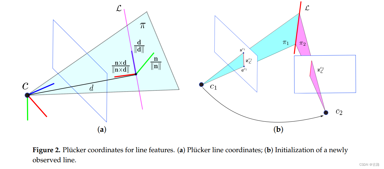
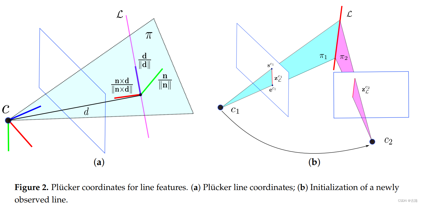
在图 $2\mathrm{a}$ 中, 普吕克坐标中的 $3\mathrm{D}$ 空间线 $\mathcal{L}$ 由 $\mathcal{L}={\left({\mathbf{n}}^{\top },{\mathrm{d}}^{\top }\right)}^{\top }\in {\mathbb{R}}^6$ 表示, 其中 $\mathrm{d}\in {\mathbb{R}}^3$ 是线方向向量, $\mathrm{n}\in {\mathbb{R}}^3$ 是由直线和坐标原点确定的平面法向量。Plücker 坐标被过度参数化，因为向量 $\mathrm{n}$ 和 $\mathrm{d}$ 之间存在隐式约束，即 ${\mathrm{n}}^{\top }\mathrm{d}=0$ 。因此, Plücker坐标不能直接用于无约束优化。然而, 使用由法线向量和方向向量表示的 3D 线, 可以简单地从两个几何视图执行三角测量, 并且也可以方便地对线几何变换进行建模。

对于线几何变换, 给定从世界坐标系 $\mathrm{w}$ 到相机坐标系 $\mathrm{c}$ 的变换矩阵 ${\mathbf{T}}_{cw}=\left[\begin{array}{cc}{\mathbf{R}}_{cw}& {\mathbf{P}}_{cw}\\ 0& 1\end{array}\right]$, 我们可以将线的 Plücker 坐标变换为 [30]
$${\mathcal{L}}^c=\left[\begin{array}{c}{\mathbf{n}}^c\\ {\mathbf{d}}^c\end{array}\right]=J_{cw}{\mathcal{L}}_w=\left[\begin{array}{cc}{\mathbf{R}}_{cw}& {\left[{\mathbf{p}}_{cw}\right]}_x{\mathbf{R}}_{cw}\\ 0& {\mathbf{R}}_{cw}\end{array}\right]{\mathcal{L}}^w$$

其中 $[\cdot {]}_{\times }$是三维向量的斜对称矩阵， $J_{cw}$ 是用于将线从帧 $w$ 变换到帧 $\mathrm{c}$ 的变换矩阵。

当在两个不同的摄像机视图中观察到新的线地标时，可以轻松计算出普吕克坐标。如图 $2\mathrm{b}$ 所示，3D 线 $\mathcal{L}$ 由摄像机 $c_1$ 和 $c_2$ 捕获为 ${\mathrm{z}}_L^{c_1}$ 和 ${\mathrm{z}}_l^{c_2}$。归一化图像平面中的线段 ${\mathrm{z}}_L^{c_1}$ 可以由两个端点 ${\mathrm{s}}^{c_1}={\left[u_s,v_s,1\right]}^T$ 和 ${\mathrm{e}}^{c_1}={\left[u_e,v_e,1\right]}^{\top }$ 表示。三个不共线的点，包括线段的两个端点和坐标原点 $\mathrm{C}={\left[x_0,y_0,z_0\right]}^{\top }$, 确定 $3\mathrm{D}$ 空间中的平面 $\pi ={\left[{\pi }_x,{\pi }_y,{\pi }_z,{\pi }_w\right]}^{\top }$ :
$${\pi }_x\left(x-x_0\right)+{\pi }_y\left(y-y_0\right)+{\pi }_z\left(z-z_0\right)=0$$
这里
$$\left[\begin{array}{c}{\pi }_x\\ {\pi }_y\\ {\pi }_z\end{array}\right]={\left[{\mathbf{s}}^{c_1}\right]}_{\times }{\mathrm{e}}^{c_1},{\pi }_w={\pi }_x{x}_0+{\pi }_y{y}_0+{\pi }_z{z}_0$$

• 这里对偶矩阵的内容可以看《多视图几何》

给定相机坐标系 $c_1$ 中的两个平面 ${\pi }_1$ 和 ${\pi }_2$, 对偶普吕克矩阵 ${\mathrm{L}}^{\ast }$ 可以通过以下方式计算
$${\mathbf{L}}^{\ast }=\left[\begin{array}{cc}[\mathbf{d}{]}_{\mathbf{x}}& \mathbf{n}\\ -{\mathbf{n}}^{\top }& 0\end{array}\right]={\pi }_1{\pi }_2^{\top }-{\pi }_2{\pi }_1^{\top }\in {\mathbb{R}}^{4\times 4}$$

相机坐标系 $c_1$ 中的 Plücker 坐标 $\mathcal{L}=({\mathbf{n}}^T,{\mathbf{d}}^T{)}^T$很容易从对偶 Plücker 矩阵 $L^{\ast }$ 中提取。可以看出, $\mathbf{n}$ 和 $\mathrm{d}$ 不需要是单位向量。

主体逻辑在void FeatureManager::triangulateLine(Vector3d Ps[], Vector3d tic[], Matrix3d ric[]) 中：

• 根据线段起点终点相机原点求平面：

/*三点确定一个平面 a(x-x0)+b(y-y0)+c(z-z0)=0  --> ax + by + cz + d = 0   d = -(ax0 + by0 + cz0)平面通过点（x0,y0,z0）以及垂直于平面的法线（a,b,c）来得到(a,b,c)^T = vector(AO) cross vector(BO)d = O.dot(cross(AO,BO))*/
Vector4d pi_from_ppp(Vector3d x1, Vector3d x2, Vector3d x3) {Vector4d pi;pi << ( x1 - x3 ).cross( x2 - x3 ), - x3.dot( x1.cross( x2 ) ); // d = - x3.dot( (x1-x3).cross( x2-x3 ) ) = - x3.dot( x1.cross( x2 ) )return pi;
}

如果两平面夹角小于 15 度，不三角化。两个平面求交线：

// 两平面相交得到直线的plucker 坐标
Vector6d pipi_plk( Vector4d pi1, Vector4d pi2){Vector6d plk;Matrix4d dp = pi1 * pi2.transpose() - pi2 * pi1.transpose();plk << dp(0,3), dp(1,3), dp(2,3), - dp(1,2), dp(0,2), - dp(0,1);return plk;
}

 Vector6d plk = pipi_plk(pii, pij);Vector3d n = plk.head(3);Vector3d v = plk.tail(3);// ...plk坐标的矩阵形式Vector3d pc, nc, vc;nc = it_per_id.line_plucker.head(3);vc = it_per_id.line_plucker.tail(3);Matrix4d Lc;Lc << skew_symmetric(nc), vc, -vc.transpose(), 0;

3.2.正交表示

由于3D空间的直线只有4个自由度，使用Plücker坐标这种过参数化的表示形式在优化的时候不方便，所以我们引入四个参数的正交表示 $(\mathbf{U},\mathbf{W})\in SO(3)\times SO(2)$ 。Plücker坐标和正交表示之间可以很方便的互相转换，我们之后会分别介绍如何从Plücker坐标到正交表示和正交表示怎么变换成Plücker坐标。首先我们需要知道了直线的Plücker坐标 $\mathcal{L}=({\mathbf{n}}^{\top },{\mathbf{d}}^{\top }{)}^{\top }$ ，然后对 $\mathcal{L}$ 进行QR分解，得到：

$\left[\begin{array}{ll}\mathbf{n}& \mathbf{d}\end{array}\right]=\left[\begin{array}{ccc}\frac{\mathbf{n}}{\Vert \mathbf{n}\Vert }& \frac{\mathbf{d}}{\Vert \mathbf{d}\Vert }& \frac{\mathbf{n}\times \mathbf{d}}{\Vert \mathbf{n}\times \mathbf{d}\Vert }\end{array}\right]\left[\begin{array}{cc}\Vert \mathbf{n}\Vert & 0\\ 0& \Vert \mathbf{d}\Vert \\ 0& 0\end{array}\right]=\mathrm{UW}$

分解得到的第一项是正交矩阵$\mathbf{U}$ ，是一个旋转矩阵。所表示的是相机坐标系到直线坐标系的旋转。其中直线坐标系的定义如下：用直线的方向向量以及直线和光心组成平面的法向量作为坐标的两个轴，再用他们叉乘得到的向量作为第三个轴，所以

$$\mathbf{U}=\mathbf{R}(\mathbf{\psi })=\left[\begin{array}{ccc}\frac{\mathbf{n}}{||\mathbf{n}||}& \frac{\mathbf{d}}{||\mathbf{d}||}& \frac{\mathbf{n}\times \mathbf{d}}{||\mathbf{n}\times \mathbf{d}||}\end{array}\right]$$

其中 $\mathbf{\psi }={\left[{\psi }_1,{\psi }_2,{\psi }_3\right]}^{\top }$ 代表的是相机坐标系到直线坐标系在 $x$ ， $y$ 和 $z$ 轴的旋转角。

到此我们得到了正交表示的第一项，第二项需要做一些小变换。由于将 （$||\mathbf{n}||,||\mathbf{d}||$） 结合之后只有一个自由度($\mathrm{W}$的秩为2），所以我们可以用三角函数矩阵参数化：

$$\begin{array}{c}\mathbf{W}=\left[\begin{array}{cc}{w}_1& -w_2\\ w_2& w_1\end{array}\right]=\left[\begin{array}{cc}\cos (\varphi )& -\sin (\varphi )\\ \sin (\varphi )& \cos (\varphi )\end{array}\right]\\ =\frac{1}{\sqrt{\left(\Vert \mathbf{n}{\Vert }^2+\Vert \mathbf{d}{\Vert }^2\right)}}\left[\begin{array}{cc}\Vert \mathbf{n}\Vert & -\Vert \mathbf{d}\Vert \\ \Vert \mathbf{d}\Vert & \Vert \mathbf{n}\Vert \end{array}\right]\end{array}$$

上式中的 $\varphi$ 是旋转角。由于坐标原点（相机光心）到3D直线的距离是 $d=\frac{||\mathbf{n}||}{||\mathbf{d}||}$ ，所以 $\mathbf{W}$ 包含了距离信息 $d$ 的。根据 $\mathbf{U}$ 和 $\mathbf{W}$ 的定义可以看出，4个自由度包括旋转的3个自由度和距离的一个自由度。在优化的时候，我们使用 $\mathcal{O}=[\psi ,\varphi {]}^{\top }$ 作为空间直线更新的最小表示。

正交表示到Plücker坐标之间的变换可以通过下面的方式计算出来：

$${\mathcal{L}}^{\prime }={\left[w_1{\mathbf{u}}_1^T,w_2{\mathbf{u}}_2^T\right]}^T=\frac{1}{\sqrt{\left(\Vert \mathbf{n}{\Vert }^2+\Vert \mathbf{d}{\Vert }^2\right)}}\mathcal{L}$$

其中 ${\mathbf{u}}_i$ 是矩阵 $\mathbf{U}$ 的第 $i$ 列、 $w_1=\cos (\varphi )$ 和 $w_2=\sin (\varphi )$ 。 ${\mathcal{L}}^{\prime }$ 和 $\mathcal{L}$ 之间存在比例因子，但它们代表相同的3D空间线。

---

• plk转正交表示

  Vector4d plk_to_orth(Vector6d plk) {Vector4d orth;Vector3d n = plk.head(3);Vector3d v = plk.tail(3);Vector3d u1 = n / n.norm();Vector3d u2 = v / v.norm();Vector3d u3 = u1.cross(u2);// todo:: use SO3orth[0] = atan2(u2(2), u3(2));orth[1] = asin(-u1(2));orth[2] = atan2(u1(1), u1(0));Vector2d w(n.norm(), v.norm());w = w / w.norm();orth[3] = asin(w(1));return orth;
  }
  

• 正交表示转plk

  Vector6d orth_to_plk(Vector4d orth) {Vector6d plk;Vector3d theta = orth.head(3);double phi = orth[3];double s1 = sin(theta[0]);double c1 = cos(theta[0]);double s2 = sin(theta[1]);double c2 = cos(theta[1]);double s3 = sin(theta[2]);double c3 = cos(theta[2]);Matrix3d R;R << c2 * c3, s1 * s2 * c3 - c1 * s3, c1 * s2 * c3 + s1 * s3, c2 * s3,s1 * s2 * s3 + c1 * c3, c1 * s2 * s3 - s1 * c3, -s2, s1 * c2, c1 * c2;double w1 = cos(phi);double w2 = sin(phi);double d = w1 / w2;  // 原点到直线的距离Vector3d u1 = R.col(0);Vector3d u2 = R.col(1);Vector3d n = w1 * u1;Vector3d v = w2 * u2;plk.head(3) = n;plk.tail(3) = v;// Vector3d Q = -R.col(2) * d;// plk.head(3) = Q.cross(v);// plk.tail(3) = v;return plk;
  }
  

优化的时候使用正交表示。这部分操作位于line_geometry.h/cpp

4.线段残差对位姿的导数

• 这一小节理论部分来自这里,当然也是来自原论文。

4.1.直线的观测模型和误差

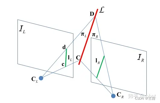
图2 空间直线投影到像素平面
要想知道线特征的观测模型，我们需要知道线特征从归一化平面到像素平面的投影内参矩阵 $\mathcal{K}$ 。如图2，点 $C$ 和 $D$ 是直线 $\mathcal{L}=({\mathbf{n}}^{\top },{\mathbf{d}}^{\top }{)}^{\top }$ 上两点，点 $c$ 和 $d$ 是它们在像素平面上的投影。 $c=KC$,$d=KD$ ,$K$是相机的内参矩阵。 $\mathbf{n}=[C{]}_{\times }D，l=\left[\begin{array}{ccc}{l}_1& l_2& l_3\end{array}\right]=[c{]}_{\times }d$ 。那么有

$$l=\mathcal{K}\mathbf{n}=\left[\begin{array}{ccc}{f}_y& 0& 0\\ 0& f_x& 0\\ -f_y{c}_x& -f_x{c}_y& f_x{f}_y\end{array}\right]\mathbf{n}$$

上式表明，直线的线投影只和法向量有关和方向向量无关。

关于投影的误差，我们不可以直接从两幅图像的线段中得到，因为同一条直线在不同图像线段的长度和大小都是不一样的。衡量线的投影误差必须从空间中重投影回当前的图像中才能定义误差。在给定世界坐标系下的空间直线 ${\mathcal{L}}_l^w$ 和正交表示 ${\mathcal{O}}_l$ ，我们首先使用 $T_{cw}=\left[\begin{array}{cc}{R}_{cw}& p_{cw}\\ 0& 1\end{array}\right]$ 将直线变换到相机 $c_i$ 坐标下。然后再将直线投影到成像平面上得到投影线段 $l_l^{c_i}$ ，然后我们就得到了线的投影误差。我们将线的投影误差定义为图像中观测线段的端点到从空间重投影回像素平面的预测直线的距离。

$$\begin{gathered} {\mathbf{r}}_l\left({\mathbf{z}}_{{\mathcal{L}}_l}^{c_i},\mathcal{X}\right)=\left[\begin{array}{l}d\left({\mathbf{s}}_l^{c_i},{\mathbf{l}}_l^{c_i}\right)\\ d\left({\mathbf{e}}_l^{c_i},{\mathbf{l}}_l^{c_i}\right)\end{array}\right] \\ d(\mathbf{s},1)=\frac{{\mathbf{s}}^{\top }\mathbf{l}}{\sqrt{l_1^2+l_2^2}} \end{gathered}$$

其中 ${\mathbf{s}}_l^{c_i}$ 和 ${\mathbf{e}}_l^{c_i}$ 是图像中观测到的线段端点， ${\mathbf{l}}_l^{c_i}$ 是重投影的预测的直线。

4.2.误差雅克比推导

如果要优化的话，需要知道误差的雅克比矩阵：

线特征在VIO下根据链式求导法则：

$${\mathbf{J}}_l=\frac{\partial {\mathbf{r}}_l}{\partial {\mathbf{l}}^{c_i}}\frac{\partial {\mathbf{l}}^{c_i}}{\partial {\mathcal{L}}^{c_i}}\left[\frac{\partial {\mathcal{L}}^{c_i}}{\partial \delta {\mathbf{x}}^i}\frac{\partial {\mathcal{L}}^{c_i}}{\partial {\mathcal{L}}^w}\frac{\partial {\mathcal{L}}^w}{\partial \delta \mathcal{O}}\right]$$

其中第一项 $\frac{\partial {\mathbf{r}}_l}{\partial {\mathbf{l}}^{c_i}}$ ，因为

$$\begin{gathered} {\mathbf{r}}_l=\left[\begin{array}{c}\frac{{\mathbf{s}}^T\mathbf{l}}{\sqrt{l_1^2+l_2^2}}\\ \frac{{\mathbf{e}}^T\mathbf{l}}{\sqrt{l_1^2+l_2^2}}\end{array}\right]=\left[\begin{array}{c}\frac{u_s{l}_1+v_s{l}_2}{\sqrt{l_1^2+l_2^2}}\\ \frac{u_e{l}_1+v_e{l}_2}{\sqrt{l_1^2+l_2^2}}\end{array}\right] \\ \mathbf{s}=\left[\begin{array}{ccc}{u}_s& v_s& 1\end{array}\right] \\ \mathbf{e}=\left[\begin{array}{ccc}{u}_e& v_e& 1\end{array}\right] \\ \mathbf{l}=\left[\begin{array}{ccc}{l}_1& l_2& l_3\end{array}\right] \end{gathered}$$

所以：

$$\begin{array}{rl}\frac{\partial {\mathbf{r}}_l}{\partial \mathbf{l}}& =\left[\begin{array}{lll}\frac{\partial r_1}{{\partial }_1}& \frac{\partial r_1}{\partial l_2}& \frac{\partial r_1}{\partial l_3}\\ \frac{\partial r_2}{\partial l_1}& \frac{\partial r_2}{\partial l_2}& \frac{\partial r_2}{\partial l_3}\end{array}\right]\\ & ={\left[\begin{array}{ccc}\frac{-l_1{\mathbf{s}}_l^{\top }\mathbf{l}}{{\left(l_1^2+l_2^2\right)}^{\left(\frac{3}{2}\right)}}+\frac{u_s}{{\left(l_1^2+l_2^2\right)}^{\left(\frac{1}{2}\right)}}& \frac{-l_2{\mathbf{s}}_l^{\top }\mathbf{l}}{{\left(l_1^2+l_2^2\right)}^{\left(\frac{3}{2}\right)}}+\frac{v_s}{{\left(l_1^2+l_2^2\right)}^{\left(\frac{1}{2}\right)}}& \frac{1}{{\left(l_1^2+l_2^2\right)}^{\left(\frac{1}{2}\right)}}\\ \frac{-l_1{\mathbf{e}}_l^{\top }\mathbf{l}}{{\left(l_1^2+l_2^2\right)}^{\left(\frac{3}{2}\right)}}+\frac{e_s}{{\left(l_1^2+l_2^2\right)}^{\left(\frac{1}{2}\right)}}& \frac{-l_2{\mathbf{e}}_l^{\top }\mathbf{l}}{{\left(l_1^2+l_2^2\right)}^{\left(\frac{3}{2}\right)}}+\frac{v_e}{{\left(l_1^2+l_2^2\right)}^{\left(\frac{1}{2}\right)}}& \frac{1}{{\left(l_1^2+l_2^2\right)}^{\left(\frac{1}{2}\right)}}\end{array}\right]}_{2\times 3}\end{array}$$

第二项 $\frac{\partial {\mathbf{l}}^{c_i}}{\partial {\mathcal{L}}^{c_i}}$ ，因为

$$\begin{gathered} \mathbf{l}=\mathcal{K}\mathbf{n} \\ \mathcal{L}=\left[\begin{array}{cc}\mathbf{n}& \mathbf{d}\end{array}\right] \end{gathered}$$

所以：

$$\begin{array}{rl}\frac{\partial {\mathrm{l}}^{c_i}}{\partial {\mathcal{L}}_i^{c_i}}& =\left[\begin{array}{cc}\frac{\partial \mathbf{l}}{\mathbf{n}}& \frac{\partial \mathbf{l}}{\mathbf{d}}\end{array}\right]\\ & ={\left[\begin{array}{ll}\mathcal{K}& 0\end{array}\right]}_{3\times 6}\end{array}$$

最后一项矩阵包含两个部分，一个是相机坐标系下线特征对的旋转和平移的误差导数，第二个是直线对正交表示的四个参数增量的导数

第一部分中，

$$\delta {\mathbf{x}}_i=\left[\delta \mathbf{p},\delta \mathbf{\theta },\delta \mathbf{v},\delta {\mathbf{b}}_a^{b_i},\delta {\mathbf{b}}_g^{b_i}\right]$$

在VIO中，如果要计算线特征的重投影误差，需要将在世界坐标系 $w$ 下的线特征变换到IMU坐标系 $b$ 下，再用外参数 ${\mathbf{T}}_{\mathbf{bc}}$ 变换到相机坐标系 $c$ 下。所以

$$\begin{array}{rl}{\mathcal{L}}_c& ={\mathcal{T}}_{bc}^{-1}{\mathcal{T}}_{wb}^{-1}{\mathcal{L}}_w\\ & ={\mathcal{T}}_{bc}^{-1}{\left[\begin{array}{c}{\mathbf{R}}_{wb}^{\top }\left({\mathbf{n}}^w+\left[{\mathbf{d}}^w\right]\times {\mathbf{p}}_{wb}\right)\\ {\mathbf{R}}_{wb}^{\top }{\mathbf{d}}^w\end{array}\right]}_{6\times 1}\end{array}$$

其中
$$\begin{gathered} {\mathcal{T}}_{bc}=\left[\begin{array}{cc}{\mathbf{R}}_{bc}& {\left[{\mathbf{p}}_{bc}\right]}_{\times }{\mathbf{R}}_{bc}\\ 0& {\mathbf{R}}_{bc}\end{array}\right] \\ {\mathcal{T}}_{bc}^{-1}=\left[\begin{array}{cc}{\mathbf{R}}_{\mathbf{bc}}^{\top }& -{\mathbf{R}}_{\mathbf{bc}}^{\top }[{\mathbf{p}}_{\mathbf{bc}}{]}_{\times }\\ 0& {\mathbf{R}}_{\mathbf{bc}}^{\top }\end{array}\right] \end{gathered}$$
$$-[a{]}_{\times }b=[b{]}_{\times }a$$
线特征 $\mathcal{L}$ 只优化状态变量中的位移和旋转，所以只需要对位移和旋转求导，其他都是零。下面我们来具体分析旋转和位移的求导。首先是线特征对旋转的求导：

$$\begin{array}{rl}\frac{\partial {\mathcal{L}}_c}{\partial \delta {\theta }_{b{b}^{\prime }}}& ={\mathcal{T}}_{bc}^{-1}\left[\begin{array}{c}\frac{\partial \left(\mathbf{I}-{\left[\delta {\mathbf{\theta }}_{b{b}^{\prime }}\right]}_{\times }\right){\mathbf{R}}_{wb}^{\top }\left({\mathbf{n}}^w+{\left[{\mathbf{d}}^w\right]}_{\times }{\mathbf{p}}_{wb}\right)}{\partial \delta {\mathbf{\theta }}_{b{b}^{\prime }}}]\\ \frac{\partial \left(\mathbf{I}-{\left[\delta {\mathbf{\theta }}_{b{b}^{\prime }}\right]}_{\times }^{\top }\right){\mathbf{R}}_{wb}^{\top }{\mathbf{d}}^w}{\partial \delta {\mathbf{\theta }}_{b{b}^{\prime }}}\end{array}\right]\\ & ={\mathcal{T}}_{bc}^{-1}{\left[\begin{array}{c}{\left[{\mathbf{R}}_{wb}^{\top }\left({\mathbf{n}}^w+{\left[{\mathbf{d}}^w\right]}_{\times }{\mathbf{p}}_{wb}\right)\right]}_{\times }]\\ {\left[{\mathbf{R}}_{wb}^{\top }{\mathbf{d}}^w\right]}_{\times }\end{array}\right]}_{6\times 3}\end{array}$$

然后是线特征对位移的求导：

$$\begin{array}{rl}\frac{\partial {\mathcal{T}}_c}{\partial \delta {\mathbf{p}}_{\mathbf{b}{\mathbf{b}}^{\prime }}}& ={\mathcal{T}}_{bc}^{-1}\left[\begin{array}{c}\frac{\partial {\mathbf{R}}_{wb}^{\top }\left({\mathbf{n}}^w+{\left[{\mathbf{d}}^w\right]}_{\times }\left({\mathbf{p}}_{wb}+\delta {\mathbf{p}}_{b{b}^{\prime }}\right)\right)}{\partial \delta {\mathbf{p}}_{b{b}^{\prime }}}\\ \frac{\partial {\mathbf{R}}_{wb}^{\top }{\mathbf{d}}^w}{\partial \delta {\mathbf{p}}_{b{b}^{\prime }}}\end{array}\right]\\ & ={\mathcal{T}}_{bc}^{-1}{\left[\begin{array}{c}{\mathbf{R}}_{wb}^{\top }{\left[{\mathbf{d}}^w\right]}_{\times }\\ 0\end{array}\right]}_{6\times 3}\end{array}$$

第二部分中 $\frac{\partial {\mathcal{L}}^{c_i}}{\partial {\mathcal{L}}^w}\frac{\partial {\mathcal{L}}^w}{\partial \delta \mathcal{O}}$ ，先解释第一个 $\frac{\partial {\mathcal{L}}^{c_i}}{\partial {\mathcal{L}}^w}$

$${\mathcal{L}}^c={\mathcal{T}}_{wc}^{-1}{\mathcal{L}}^w$$

所以 $\frac{\partial {\mathcal{L}}^{c_i}}{\partial {\mathcal{L}}^w}={\mathcal{T}}_{wc}^{-1}$

然后后面的 $\frac{\partial {\mathcal{L}}^w}{\partial \delta \mathcal{O}}$ 有两种思路，先介绍第一种：

$$\begin{gathered} \frac{\partial {\mathcal{L}}^w}{\partial \delta \mathcal{O}}=\left[\begin{array}{cccc}\frac{\partial {\mathcal{L}}^w}{\partial {\psi }_1}& \frac{\partial {\mathcal{L}}^w}{\partial {\psi }_2}& \frac{\partial {\mathcal{L}}^w}{\partial {\psi }_3}& \frac{\partial {\mathcal{L}}^w}{\partial \varphi }\end{array}\right] \\ \frac{\partial {\mathcal{L}}^w}{\partial {\psi }_1}=\frac{\partial {\mathcal{L}}^w}{\partial \mathbf{U}}\frac{\partial \mathbf{U}}{\partial {\psi }_1} \\ \frac{\partial {\mathcal{L}}^w}{\partial \varphi }=\frac{\partial {\mathcal{L}}^w}{\partial \mathbf{w}}\frac{\partial \mathbf{w}}{\partial {\varphi }_1} \end{gathered}$$

其中 $\mathcal{L}$ 对 $\mathbf{U}$ 和 $\mathbf{w}=[w_1,w_2]$ 求导，因为 ${\mathcal{L}}^w={\left[\begin{array}{cc}{w}_1{\mathbf{u}}_1^{\top }& w_2{\mathbf{u}}_2^{\top }\end{array}\right]}^{\top }$ ，所以

$$\begin{array}{rl}\frac{\partial \mathcal{L}}{\partial \mathbf{U}}& ={\left[\begin{array}{ccc}\frac{\partial \mathcal{L}}{\partial {\mathbf{U}}_1}& \frac{\partial \mathcal{L}}{\partial {\mathbf{U}}_2}& \frac{\partial \mathcal{L}}{\partial {\mathbf{U}}_3}\end{array}\right]}_{6\times 9}\\ & =\left[\begin{array}{ccc}{w}_{1(3\times 3)}& 0& 0\\ 0& w_{2(3\times 3)}& 0\end{array}\right]\end{array}$$

$$\begin{array}{rl}\frac{\partial \mathcal{L}}{\partial \mathbf{w}}& ={\left[\begin{array}{cc}\frac{\partial \mathcal{L}}{\partial w_1}& \frac{\partial \mathcal{L}}{\partial w_2}\end{array}\right]}_{6\times 2}\\ & =\left[\begin{array}{cc}{\mathbf{u}}_1& 0\\ 0& {\mathbf{u}}_2\end{array}\right]\end{array}$$

然后是 $\mathbf{U}$ 对 $\psi$ 和 $\mathbf{W}$ 对 $\varphi$ 的求导，

因为 $\begin{array}{rl}{\mathbf{U}}^{\prime }& \approx \mathbf{U}\left(\mathbf{I}+[\delta \psi {]}_{\times }\right)\end{array}$ ，所以

$$\begin{gathered} {\left[\begin{array}{ccc}{\mathbf{u}}_1& {\mathbf{u}}_2& {\mathbf{u}}_3\end{array}\right]}^{\prime }=\left[\begin{array}{ccc}{\mathbf{u}}_1& {\mathbf{u}}_2& {\mathbf{u}}_3\end{array}\right]+{\left[\begin{array}{ccc}{\mathbf{u}}_1& {\mathbf{u}}_2& {\mathbf{u}}_3\end{array}\right]}_{\times }\delta \psi \\ \frac{{\left[\begin{array}{ccc}{\mathbf{u}}_1& {\mathbf{u}}_2& {\mathbf{u}}_3\end{array}\right]}^{\prime }-\left[\begin{array}{ccc}{\mathbf{u}}_1& {\mathbf{u}}_2& {\mathbf{u}}_3\end{array}\right]}{\delta \psi }={\left[\begin{array}{ccc}{\mathbf{u}}_1& {\mathbf{u}}_2& {\mathbf{u}}_3\end{array}\right]}_{\times } \\ \frac{\partial \mathbf{U}}{\partial {\psi }_1}=\left[\begin{array}{ccc}0& {\mathbf{u}}_3& -{\mathbf{u}}_2\end{array}\right] \\ \frac{\partial \mathbf{U}}{\partial {\psi }_2}=\left[\begin{array}{ccc}-{\mathbf{u}}_3& 0& {\mathbf{u}}_1\end{array}\right] \\ \frac{\partial \mathbf{U}}{\partial {\psi }_1}=\left[\begin{array}{ccc}{\mathbf{u}}_2& -{\mathbf{u}}_1& 0\end{array}\right] \\ \frac{\partial \mathbf{w}}{\partial \varphi }=\left[\begin{array}{c}-w_2\\ w_1\end{array}\right] \end{gathered}$$

所以，可得

$$\begin{array}{rl}\frac{\partial {\mathcal{L}}^w}{\partial \delta \mathcal{O}}& =\left[\begin{array}{cccc}\frac{\partial {\mathcal{L}}^w}{\partial {\psi }_1}& \frac{\partial {\mathcal{L}}^w}{\partial {\psi }_2}& \frac{\partial {\mathcal{L}}^w}{\partial {\psi }_3}& \frac{\partial {\mathcal{L}}^w}{\partial \varphi }\end{array}\right]\\ & =\left[\begin{array}{cccc}\frac{\partial {\mathcal{L}}^w}{\partial \mathbf{U}}\frac{\partial \mathbf{U}}{\partial {\psi }_1}& \frac{\partial {\mathcal{L}}^w}{\partial \mathbf{U}}\frac{\partial \mathbf{U}}{\partial {\psi }_2}& \frac{\partial {\mathcal{L}}^w}{\partial \mathbf{U}}\frac{\partial \mathbf{U}}{\partial {\psi }_3}& \frac{\partial {\mathcal{L}}^w}{\partial \mathbf{w}}\frac{\partial \mathbf{w}}{\partial \varphi }\end{array}\right]\\ & ={\left[\begin{array}{cccc}0& -w_1{\mathbf{u}}_3& w_1{\mathbf{u}}_2& -w_2{\mathbf{u}}_1\\ w_2{\mathbf{u}}_3& 0& -w_2{\mathbf{u}}_1& w_1{\mathbf{u}}_2\end{array}\right]}_{6\times 4}\end{array}$$

---

todo:代码阅读