题目

赛题描述

给定企业客户信息，建立分类模型，判断企业客户是否会流失。

数据说明

数据主要包括企业客户样本信息。 数据分为训练数据和测试数据，分别保存在train.csv和test_noLabel.csv两个文件中。 字段说明如下：
（1）ID：编号
（2）Contract：是否有合同
（3）Dependents：是否有家属
（4）DeviceProtection：是否有设备保护
（5）InternetService：是否有互联网服务
（6）MonthlyCharges：月度费用
（7）MultipleLines：是否有多条线路
（8）Partner：是否有配偶
（9）PaymentMethod：付款方式
（10）PhoneService：是否有电话服务
（11）SeniorCitizen：是否为老年人
（12）TVProgram：是否有电视节目
（15）TotalCharges：总费用
（16）gender：用户性别
（17）tenure：任期年数
（18）Churn：用户是否流失
如遇数据下载打开乱码问题： 不要用excel打开,用notepad++或者vs code。文件格式是通用的编码方式utf-8。

赛题来源-DataCastle

https://challenge.datacastle.cn/v3/cmptDetail.html?id=356

数据可在网站上下载

问题描述

通过题目给定的企业客户信息，选择适当的分类算法，建立多个分类模型，使用准确率指标评估模型性能，准确率越高，说明正确预测出企业客户流失情况的效果越好，以此找到最优的分类模型用于预测企业客户是否会流失。通过模型可以帮助企业更好地了解客户流失的趋势，从而采取相应的措施来维护客户关系。

解题思路

数据预处理：

1.检查处理缺失值、重复值、异常值
2.标签编码转化

数据可视化：
3. 各标签对流失率的影响
4. 相关性热力图绘制

建立分类模型与对比模型：
朴素贝叶斯、AdaBoost、逻辑回归、KNN、SVM、
随机森林、XGBoost、MLP、 LightGBM、GBDT、
随机森林-MLP-XGBoost组合模型

使用随机搜索及贝叶斯优化 进行超参数调优

Python实现

读取数据并初步了解

导入宏包

import pandas as pd
import numpy as np
import matplotlib.pyplot as plt
import seaborn as sns
from scipy import stats
from scipy.special import boxcox1p
import missingno as msno
import warnings
warnings.filterwarnings("ignore")
%matplotlib inline

读取数据

train = pd.read_csv('train.csv')
test = pd.read_csv('test_noLabel.csv')
train.shape,test.shape

train.head()
test.head()

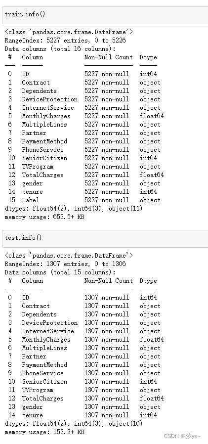
查看数据类型

train.info()
test.info()

检查缺失值

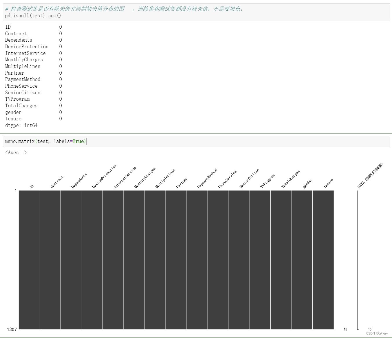
使用 pd.isnull(train).sum() 查看缺失值情况。并通过 msno.matrix() 绘制缺失值热力图，从结果可以看出数据集不存在缺失值

# 检查训练集是否有缺失值并绘制缺失值分布的图,无缺失值
pd.isnull(train).sum()msno.matrix(train, labels=True)

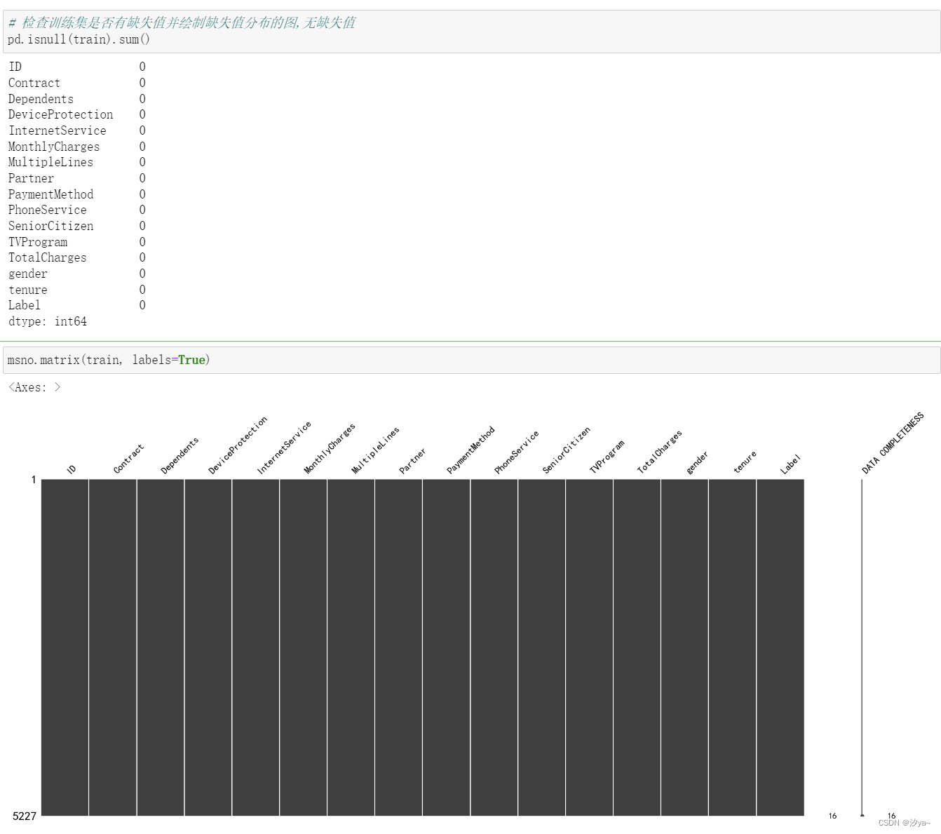
# 检查测试集是否有缺失值并绘制缺失值分布的图   ，训练集和测试集都没有缺失值，不需要填充。
pd.isnull(test).sum()
msno.matrix(test, labels=True)

描述性统计分析

使用 train.describe().T 对数值型列进行描述性统计分析，包括平均值、标准差、最大值、最小值等。

train.describe()
test.describe()

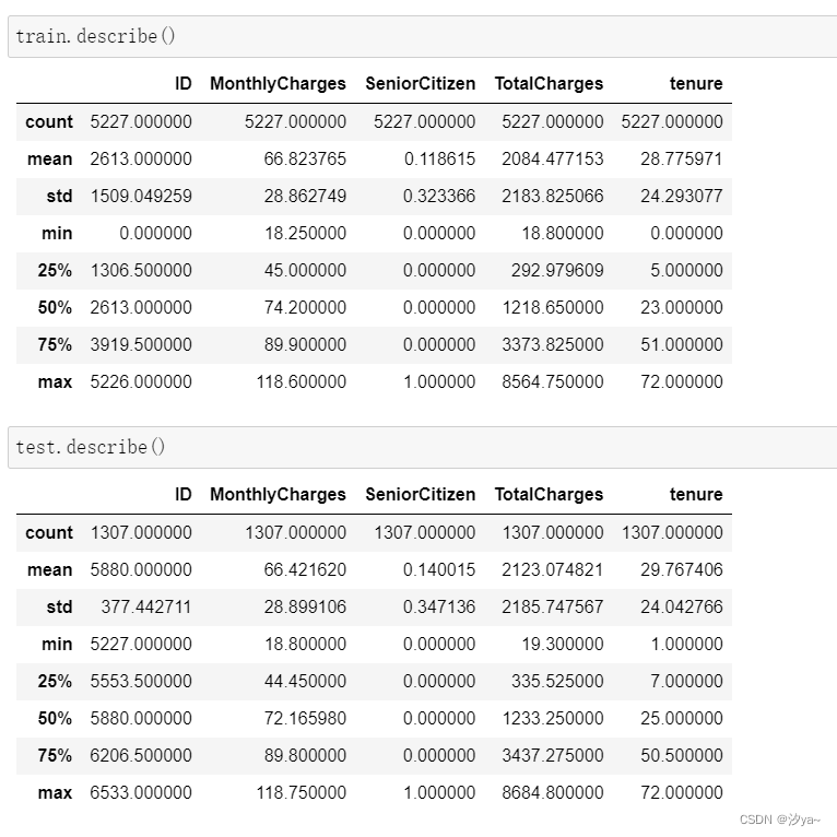
这份数据描述统计结果提供了关于客户信息的多个方面的信息。其中包括每月费用的平均值约为66.82，老年人占比约为11.86%，客户的平均任期约为 28.78个月，以及总费用的平均值约为2084.48。这些数据能够描绘出客户的消费情况、老年人比例以及服务使用时长等信息，另外提供查看最大最小 值，可以初步确定数据无逻辑异常。

可视化分析

用户流失分析

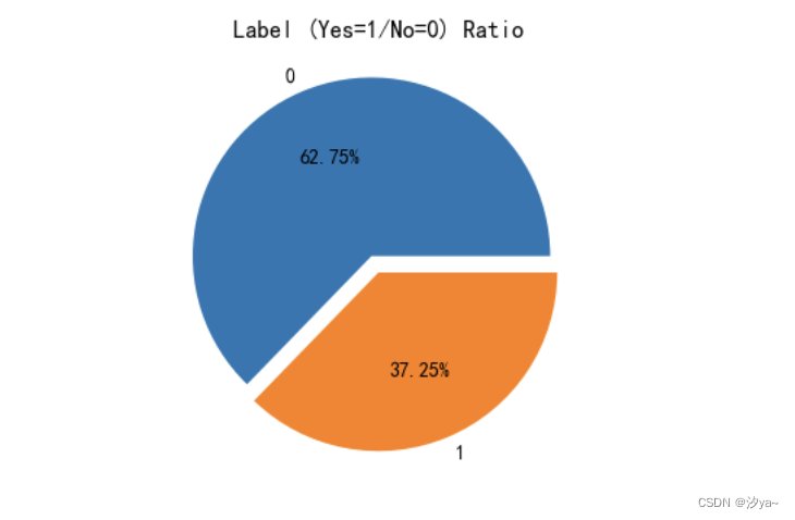
使用 train['Label'].value_counts() 统计不同标签（流失与否）的数量。并绘制了用户流失比例的扇形图和不同特征对客户流失率的影响的柱状 图。通过结果可以看出数据集中有62.75%用户没流失，337.25%客户流失，数据集是不均衡。

#流失用户数量和占比
import matplotlib.pyplot as plt
plt.rcParams['figure.figsize'] = 4, 4
plt.pie(train['Label'].value_counts(), labels=train['Label'].value_counts().index, autopct='%1.2f%%', explode=(0.1, 0))
plt.title('Label (Yes=1/No=0) Ratio')
plt.show()

特征分析

#用户属性柱状图
import seaborn as sns
import matplotlib.pyplot as plt# 设置中文字体为 SimHei
plt.rcParams['font.sans-serif'] = ['SimHei']
plt.rcParams['axes.unicode_minus'] = False  # 解决负号显示问题# 设置图表尺寸
plt.rcParams['figure.figsize'] = (12, 10)# 绘制性别对客户流失率的影响
plt.subplot(2, 2, 1)
sns.countplot(x='gender', hue='Label', data=train)
plt.title('性别对客户流失率的影响')# 绘制老人对客户流失率的影响
plt.subplot(2, 2, 2)
sns.countplot(x='SeniorCitizen', hue='Label', data=train)
plt.title('老人对客户流失率的影响')# 绘制配偶对客户流失率的影响
plt.subplot(2, 2, 3)
sns.countplot(x='Partner', hue='Label', data=train)
plt.title('配偶对客户流失率的影响')# 绘制亲属对客户流失率的影响
plt.subplot(2, 2, 4)
sns.countplot(x='Dependents', hue='Label', data=train)
plt.title('亲属对客户流失率的影响')# 显示图表
plt.show()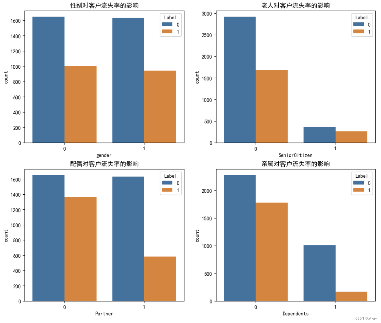

对于性别、老人、配偶、亲属等特征，使用 sns.countplot() 绘制柱状图，分析其对客户流失率的影响。
可以得出下面结论：
1. 性别对用户流失影响不大；
2. 年轻用户的流失率显著高于年长用户；
3. 有伴侣的用户流失比例低于无伴侣用户；
4. 用户中有家属的数量较少；
5. 有家属的用户流失比例低于无家属用户。

任期年数与客户流失的关系：

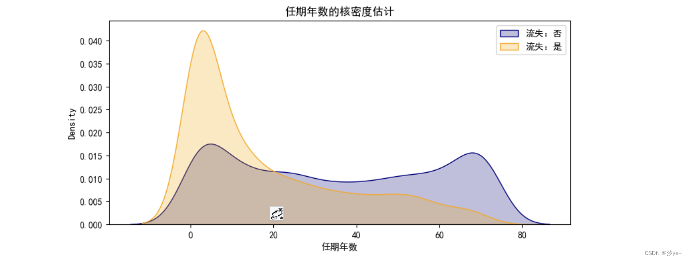
使用 sns.kdeplot() 绘制核密度估计图，在网时长越久，流失率越低，符合一般经验；在网时间达到三个月，流失率小于在网率，证明用户心理稳定 期一般是三个月。

import seaborn as sns
import matplotlib.pyplot as plt# 设置中文字体为 SimHei
plt.rcParams['font.sans-serif'] = ['SimHei']
plt.rcParams['axes.unicode_minus'] = False  # 解决负号显示问题# Kernel density estimaton核密度估计
def kdeplot(feature, xlabel, df):plt.figure(figsize=(9, 4))plt.title("{0}的核密度估计".format(xlabel))  # 中文标题ax0 = sns.kdeplot(df[df['Label'] == 'No'][feature].dropna(), color='navy', label='流失：否', shade='True')ax1 = sns.kdeplot(df[df['Label'] == 'Yes'][feature].dropna(), color='orange', label='流失：是', shade='True')plt.xlabel(xlabel)plt.legend(fontsize=10)# 调用函数绘制核密度图
kdeplot('tenure', '任期年数',train )
plt.show()# 在网时长越久，流失率越低，符合一般经验；
# 在网时间达到三个月，流失率小于在网率，证明用户心理稳定期一般是三个月。# 这个核密度估计图展示了用户任期年数 (`tenure`) 与客户流失 (`Label`) 的关系。在这张图中：# - **横轴 (`tenure`):** 表示用户的任期年数。这个轴展示了用户在服务提供商（可能是电信公司等）停留的时间跨度。# - **纵轴（密度）:** 表示在每个任期年数上流失与不流失客户的密度估计。密度估计通常显示了不同任期年数上客户流失的相对频率。在这里，越高的密度意味着在特定的任期年数上，流失或不流失的用户数量较多。# - **曲线:** 图中有两条曲线，一条代表流失为 "No"（蓝色），另一条代表流失为 "Yes"（橙色）。这两条曲线代表了任期年数对于流失与否的概率密度分布。当曲线较高的区域重叠时，表示在这些任期年数上流失与不流失的用户数量相近；而当曲线差异较大时，则代表在该任期年数上流失和不流失的用户数量有显著差异。# 这个图可以帮助你理解在不同的任期年数下，用户流失和不流失的趋势。例如，你可以观察到在哪些任期年数上流失率较高或较低，以及是否存在明显的任期年数区间，对流失率有重要影响。

服务类属性分析

#服务属性分析
import seaborn as sns
import matplotlib.pyplot as plt
# 设置中文字体为 SimHei
plt.rcParams['font.sans-serif'] = ['SimHei']
plt.rcParams['axes.unicode_minus'] = False  # 解决负号显示问题# 设置图表尺寸
plt.figure(figsize=(10, 5))# 绘制 MultipleLines 对用户流失的影响的柱状图
plt.subplot(1, 2, 1)  # 创建第一个子图
sns.countplot(x='MultipleLines', hue='Label', data=train)
plt.title('多条线路对用户流失的影响')
plt.xlabel('是否有多条线路')
plt.ylabel('用户数量')
plt.legend(title='流失')# 绘制 InternetService 对用户流失的影响的柱状图
plt.subplot(1, 2, 2)  # 创建第二个子图
sns.countplot(x='InternetService', hue='Label', data=train)
plt.title('互联网服务对用户流失的影响')
plt.xlabel('是否有互联网服务')
plt.ylabel('用户数量')
plt.legend(title='流失')# 调整子图布局
plt.tight_layout()# 显示图表
plt.show()

使用 sns.countplot() 分析不同服务属性对用户流失的影响，如多条线路和互联网服务。
电话服务整体对用户流失影响较大。
单光纤用户的流失占比较高；
光纤用户绑定了安全、备份、保护、技术支持服务的流失率较低；
光纤用户附加流媒体电视、电影服务的流失率占比较低。

特征相关性分析

import numpy as np
import matplotlib.pyplot as plt
import seaborn as sns# 生成关联矩阵，排除 "ID" 列
corr = train.corr()# 创建掩码矩阵
mask = np.triu(np.ones_like(corr, dtype=bool))# 创建图表
f, ax = plt.subplots(figsize=(20, 15))# 选择调色板
cmap = sns.diverging_palette(220, 10, as_cmap=True)# 绘制热力图（半三角）
plt.title('Correlation Matrix', fontsize=18)
sns.heatmap(corr, mask=mask, cmap=cmap, vmax=.3, center=0, square=True, linewidths=.5, cbar_kws={"shrink": .5}, annot=True)plt.show()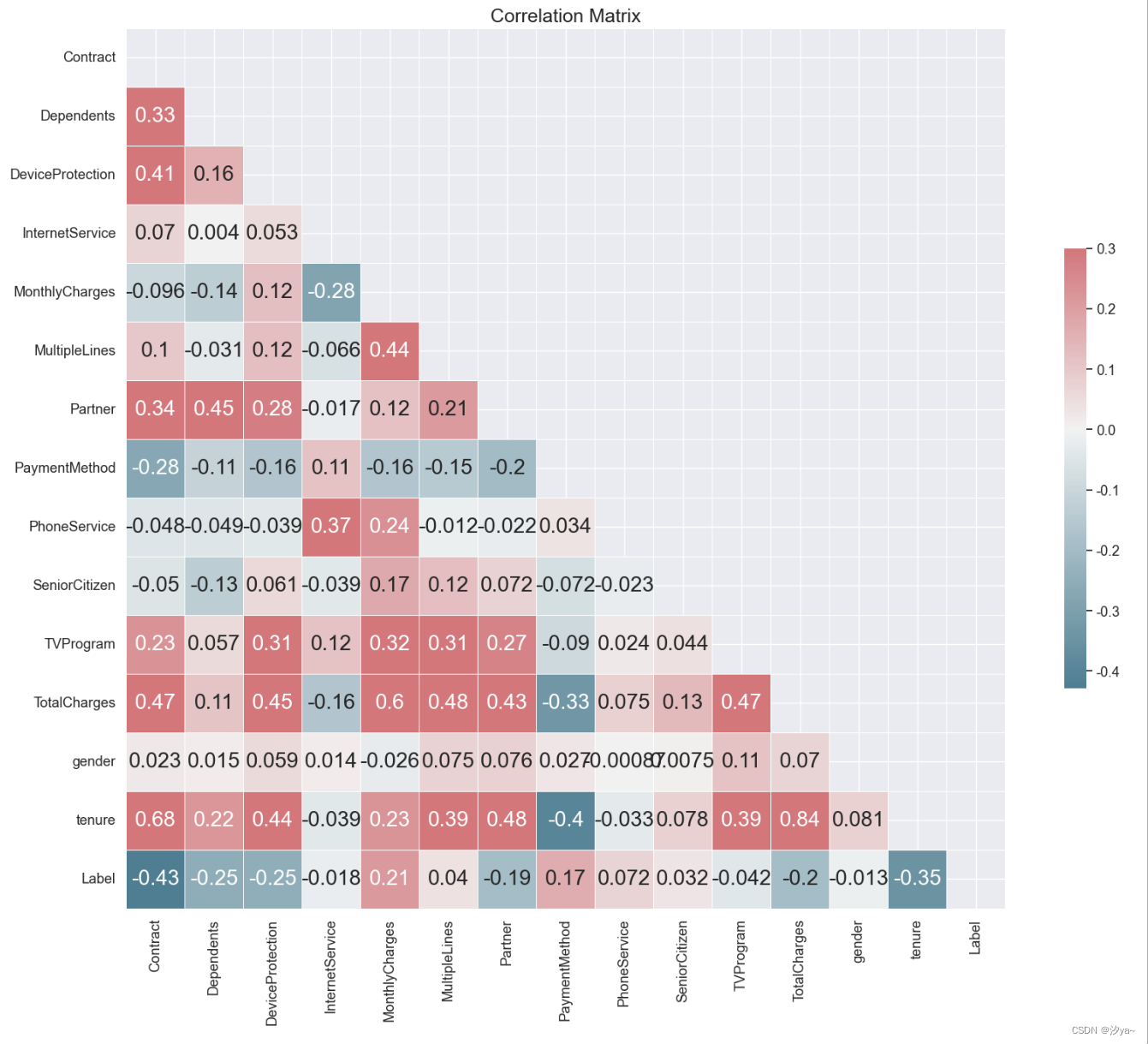

数据预处理

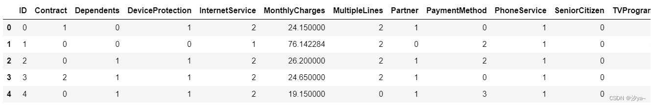
类别编码转换

from sklearn.preprocessing import LabelEncodercolumns_to_encode = ['Contract', 'Dependents', 'DeviceProtection', 'InternetService', 'MultipleLines', 'Partner', 'PaymentMethod', 'PhoneService', 'TVProgram', 'gender']for column in columns_to_encode:label_encoder = LabelEncoder()# 合并训练集和测试集的数据进行拟合combined_data = pd.concat([train[column], test[column]])label_encoder.fit(combined_data)# 对训练集进行映射train[column] = label_encoder.transform(train[column])test[column] = label_encoder.transform(test[column])# 初始化LabelEncoder并对训练集中的标签列进行映射
label_encoder = LabelEncoder()
train['Label'] = label_encoder.fit_transform(train['Label'])train.head()

划分训练数据与测试数据

train.drop('ID', axis=1, inplace=True)
test.drop('ID', axis=1, inplace=True)

# 提取特征数据与目标数据
train_noLabel = train.iloc[:, :-1]  # 选择除最后一列外的所有列作为特征
y= train['Label']  # 标签列

# 把train数据划分成80％训练数据跟20%测试数据
from sklearn.model_selection import train_test_split
x_train,x_test,y_train,y_test = train_test_split(train_noLabel,y,test_size=0.2)
print("x_train shape:", x_train.shape, "x_test shape:", x_test.shape, "y_train shape:", y_train.shape, "y_test shape:", y_test.shape)

归一化处理

from sklearn.preprocessing import MinMaxScaler# 需要归一化的列
columns_to_normalize = ['MonthlyCharges', 'TotalCharges', 'tenure']# 初始化MinMaxScaler
scaler = MinMaxScaler()# 对训练集中的指定列进行归一化
x_train[columns_to_normalize] = scaler.fit_transform(x_train[columns_to_normalize])# 对测试集中的相同列进行归一化
x_test[columns_to_normalize] = scaler.transform(x_test[columns_to_normalize])
test[columns_to_normalize] = scaler.transform(test[columns_to_normalize])

模型建立

逻辑回归

from sklearn.linear_model import LogisticRegression
from sklearn.model_selection import RandomizedSearchCV, GridSearchCV
from sklearn.metrics import accuracy_score
from scipy.stats import uniform# 定义逻辑回归模型
base_model = LogisticRegression()# 超参数调优——随机搜索#定义超参数搜索空间
param_dist = {'C': uniform(loc=1, scale=5), 'max_iter': [100, 200, 300, 400, 500]}#进行随机搜索
random_search = RandomizedSearchCV(base_model, param_distributions=param_dist, n_iter=10, cv=5, scoring='accuracy', random_state=42, n_jobs=-1)
random_search.fit(x_train, y_train)# 输出随机搜索的最佳超参数
print("随机搜索最佳超参数:", random_search.best_params_)# 获取随机搜索的最佳模型
best_model_random = random_search.best_estimator_# 进行预测和评估
predictions_random = best_model_random.predict(x_test)
accuracy_random = accuracy_score(y_test, predictions_random)
report_random = classification_report(y_test, predictions_random)
print(f"模型准确率：{accuracy_random}")# 超参数调优——网格搜索
#定义超参数搜索空间
param_grid = {'C': [0.001, 0.01, 0.1, 1, 10, 100, 1000], 'max_iter': range(1, 110, 10), 'penalty': ['l1', 'l2']}#进行网格搜索
grid_search = GridSearchCV(base_model, param_grid, cv=5, scoring='accuracy')
grid_search.fit(x_train, y_train)# 输出网格搜索的最佳超参数
print("网格搜索最佳超参数:", grid_search.best_params_)# 获取网格搜索的最佳模型
best_model_grid = grid_search.best_estimator_# 进行预测和评估
predictions_grid = best_model_grid.predict(x_test)
accuracy_grid = accuracy_score(y_test, predictions_grid)
report_grid = classification_report(y_test, predictions_grid)
print(f"模型准确率：{accuracy_grid}")

支持向量机（SVM）

from sklearn.svm import SVC
from sklearn.model_selection import RandomizedSearchCV
from scipy.stats import loguniform# 定义超参数搜索空间
param_dist = {'C': loguniform(1e-3, 1e3),  # 正则化参数C的对数均匀分布'gamma': loguniform(1e-3, 1e3),  # 核函数的参数gamma的对数均匀分布'kernel': ['linear', 'rbf'],  # 核函数的选择'probability': [True],  # 是否启用概率估计'random_state': [42],  # 随机种子，确保结果可重现
}# 初始化支持向量机模型
base_model = SVC()# 初始化随机搜索
random_search = RandomizedSearchCV(base_model,param_distributions=param_dist,n_iter=10,  # 设置迭代次数cv=5,  # 交叉验证折数scoring='accuracy',  # 评估指标random_state=42,  # 随机种子，确保结果可重现n_jobs=-1  # 使用所有可用的CPU核心
)# 执行随机搜索
random_search.fit(x_train, y_train)# 输出最佳参数
print("随机搜索最佳超参数: ", random_search.best_params_)# 获取最佳模型
best_model = random_search.best_estimator_# 进行预测
predictions = best_model.predict(x_test)# 评估最佳模型
accuracy = accuracy_score(y_test, predictions)
report = classification_report(y_test, predictions)print(f"模型准确率：{accuracy}")

K近邻（KNN）

from sklearn.model_selection import RandomizedSearchCV, GridSearchCV
from sklearn.neighbors import KNeighborsClassifier
from sklearn.metrics import accuracy_score# 定义KNN模型
knn_model = KNeighborsClassifier()# 超参数调优——随机搜索
# 定义参数搜索空间
param_space = {'n_neighbors': range(1, 31),  # 邻居数量范围'weights': ['uniform', 'distance'],  # 权重参数'p': [1, 2],  # 距离度量参数
}# 定义随机搜索CV对象
random_search = RandomizedSearchCV(knn_model, param_distributions=param_space, n_iter=20, cv=5, scoring='accuracy', random_state=42, n_jobs=-1)# 进行随机搜索
random_search.fit(x_train, y_train)# 输出最佳参数
best_params_random = random_search.best_params_
print("随机搜索最佳超参数：", best_params_random)# 使用最佳参数的模型进行预测和评估
best_knn_model_random = random_search.best_estimator_
predictions_random = best_knn_model_random.predict(x_test)
accuracy_random = accuracy_score(y_test, predictions_random)
report_random = classification_report(y_test, predictions_random)print(f"模型准确率：{accuracy_random}")# 超参数调优——网格搜索
# 定义超参数的范围
param_grid = {'n_neighbors': list(range(1, 30, 1)),  # 尝试不同的邻居数量'weights': ['uniform', 'distance'],  # 尝试不同的权重'p': [1, 2]  # 尝试不同的距离度量
}# 使用GridSearchCV进行超参数调优
grid_search = GridSearchCV(knn_model, param_grid, cv=5, scoring='accuracy')
grid_search.fit(x_train, y_train)# 输出最佳超参数组合
best_params_grid = grid_search.best_params_
print(f"网格搜索最佳超参数：{best_params_grid}")# 使用最佳超参数训练最终模型
best_knn_model_grid = grid_search.best_estimator_
best_knn_model_grid.fit(x_train, y_train)# 进行预测和评估
best_predictions_grid = best_knn_model_grid.predict(x_test)
best_accuracy_grid = accuracy_score(y_test, best_predictions_grid)
best_report_grid = classification_report(y_test, best_predictions_grid)print(f"模型准确率：{best_accuracy_grid}")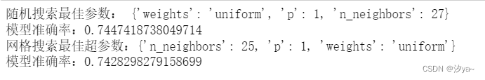

XGBoost-贝叶斯搜索超参数调优

from xgboost import XGBClassifier
from sklearn.metrics import accuracy_score
from sklearn.model_selection import train_test_split
from bayes_opt import BayesianOptimization# 定义贝叶斯优化的目标函数
def xgb_cv(learning_rate, n_estimators, max_depth, min_child_weight, subsample, gamma):xgb_model = XGBClassifier(learning_rate=learning_rate,n_estimators=int(n_estimators),max_depth=int(max_depth),min_child_weight=int(min_child_weight),subsample=subsample,gamma=gamma,random_state=42)xgb_model.fit(x_train, y_train)predictions = xgb_model.predict(x_test)accuracy = accuracy_score(y_test, predictions)return accuracy# 超参数搜索范围
param_bounds = {'learning_rate': (0.001, 0.5 ),'n_estimators': (50, 300),'max_depth': (3, 20),'min_child_weight': (1, 30),'subsample': (0.1, 1),'gamma': (0, 5)
}# 初始化贝叶斯优化对象
xgb_bayesian = BayesianOptimization(f=xgb_cv, pbounds=param_bounds, random_state=42)# 执行贝叶斯优化
xgb_bayesian.maximize(init_points=5, n_iter=100)# 输出最佳超参数
best_params = xgb_bayesian.max['params']
print("贝叶斯搜素最佳超参数：", best_params)# 使用最佳超参数构建最终模型
best_xgb_model = XGBClassifier(learning_rate=best_params['learning_rate'],n_estimators=int(best_params['n_estimators']),max_depth=int(best_params['max_depth']),min_child_weight=int(best_params['min_child_weight']),subsample=best_params['subsample'],gamma=best_params['gamma'],random_state=42
)# 训练最终模型
best_xgb_model.fit(x_train, y_train)# 进行预测
predictions = best_xgb_model.predict(x_test)# 评估最终模型
accuracy = accuracy_score(y_test, predictions)
report = classification_report(y_test, predictions)print(f"最佳模型准确率：{accuracy}")

随机森林（Random Forest）

from sklearn.ensemble import RandomForestClassifier
from sklearn.metrics import accuracy_score, classification_report
from sklearn.model_selection import train_test_split
from bayes_opt import BayesianOptimization# 数据集划分（如果没有的话）
# X_train, X_test, y_train, y_test = train_test_split(X, y, test_size=0.2, random_state=42)# 定义贝叶斯优化的目标函数
def rf_cv(n_estimators, max_depth, min_samples_split, min_samples_leaf):rf_model = RandomForestClassifier(n_estimators=int(n_estimators),max_depth=int(max_depth),min_samples_split=int(min_samples_split),min_samples_leaf=int(min_samples_leaf),random_state=42)rf_model.fit(x_train, y_train)predictions = rf_model.predict(x_test)accuracy = accuracy_score(y_test, predictions)return accuracy# 定义超参数的搜索范围
param_bounds = {'n_estimators': (50, 150),'max_depth': (3, 20),'min_samples_split': (2, 20),'min_samples_leaf': (1, 10)
}# 初始化贝叶斯优化对象
rf_bayesian = BayesianOptimization(f=rf_cv, pbounds=param_bounds, random_state=42)# 执行贝叶斯优化
rf_bayesian.maximize(init_points=5, n_iter=100)# 输出最佳超参数
best_params = rf_bayesian.max['params']
print("最佳超参数：", best_params)# 使用最佳超参数构建最终模型
best_rf_model = RandomForestClassifier(n_estimators=int(best_params['n_estimators']),max_depth=int(best_params['max_depth']),min_samples_split=int(best_params['min_samples_split']),min_samples_leaf=int(best_params['min_samples_leaf']),random_state=42
)# 训练最终模型
best_rf_model.fit(x_train, y_train)# 进行预测
predictions = best_rf_model.predict(x_test)# 评估最终模型
accuracy = accuracy_score(y_test, predictions)
report = classification_report(y_test, predictions)print(f"最佳模型准确率：{accuracy}")
print(f"最佳分类报告：\n{report}")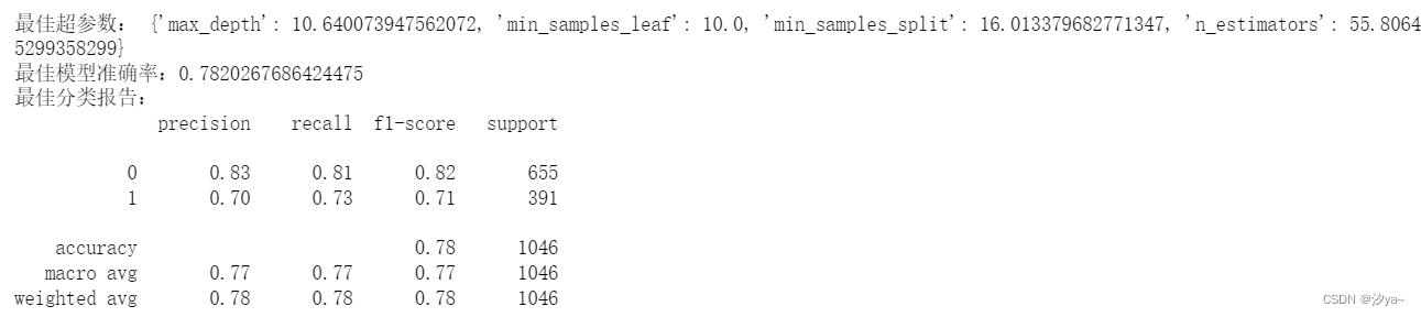

对测试集进行预测 并提交网站

# 进行预测
test_lable = best_rf_model.predict(test)  # 使用最佳模型进行测试数据集的预测
submit_example = pd.read_csv('submit_example.csv')  # 读取提交示例文件
# 替换 submit_example 的 Label 列
submit_example['Label'] = test_lable  # 将预测结果填入 submit_example 的 Label 列
submit_example['Label'] = label_encoder.inverse_transform(submit_example['Label'])  # 对 Label 进行反向转换
# 将结果写入 CSV 文件
submit_example.to_csv('Random Forest_predict.csv', index=False)  # 将结果保存为 CSV 文件，不保存索引列

AdaBoost

from sklearn.ensemble import AdaBoostClassifier
from sklearn.metrics import accuracy_score, classification_report# 初始化 AdaBoost 分类器
adaboost_model = AdaBoostClassifier(n_estimators=300, random_state=42,learning_rate=0.1)# 训练模型
adaboost_model.fit(X_train, y_train)# 进行预测
predictions = adaboost_model.predict(X_test)# 评估模型
accuracy = accuracy_score(y_test, predictions)
report = classification_report(y_test, predictions)print(f"模型准确率：{accuracy}")
print(f"分类报告：\n{report}")

MLP

from sklearn.neural_network import MLPClassifier
from sklearn.metrics import accuracy_score, classification_report# 初始化MLP模型
mlp = MLPClassifier(hidden_layer_sizes=(128, ), max_iter=100, alpha=1e-4,solver='adam', verbose=10, tol=1e-4, random_state=42,learning_rate_init=0.01)# 训练模型
mlp.fit(X_train, y_train)# 进行预测
predictions = mlp.predict(X_test)# 评估模型
accuracy = accuracy_score(y_test, predictions)
report = classification_report(y_test, predictions)print(f"模型准确率：{accuracy}")
print(f"分类报告：\n{report}")

朴素贝叶斯分类器

import pandas as pd
import numpy as np
from sklearn.model_selection import train_test_split
from sklearn.naive_bayes import GaussianNB
from sklearn.metrics import accuracy_score
from sklearn.pipeline import Pipeline# 加载数据集
def load_data(file_path):df = pd.read_csv(file_path)X = df.drop('Label', axis=1)  # 特征y = df['Label']  # 标签return X.values, y.valuesdef test_data(file_path):x = pd.read_csv(file_path)return x.values# 计算高斯概率密度函数
def gaussian_probability(x, mean, std):exponent = np.exp(-((x - mean) ** 2 / (2 * std ** 2)))   # 计算高斯分布的指数部分return (1 / (np.sqrt(2 * np.pi) * std)) * exponent     # 计算高斯概率密度函数的值# 计算类别先验概率
def calculate_class_priors(y):classes, counts = np.unique(y, return_counts=True)   # 获取标签 y 中的唯一类别和每个类别的出现次数priors = {}for c, count in zip(classes, counts):priors[c] = count / len(y)   # 计算先验概率，即该类别出现的次数除以总样本数，键为类别 'c'return priors# 计算每个特征的均值和标准差
def calculate_mean_std(X, y):class_values = list(np.unique(y))    # 获取标签y中的唯一类别，并转为列表。summaries = {}for class_value in class_values:X_class = X[y == class_value]summaries[class_value] = [(np.mean(attribute), np.std(attribute)) for attribute in X_class.T]  # 计算当前类别中每个特征的均值和标准差，并存储在字典中return summaries# 训练高斯朴素贝叶斯模型
def train_naive_bayes(X_train, y_train):priors = calculate_class_priors(y_train)summaries = calculate_mean_std(X_train, y_train)return priors, summaries# 高斯朴素贝叶斯分类器预测
def predict(priors, summaries, X_test):predictions = []   # 用于存储预测结果for row in X_test:probabilities = {}   # 用于存储每个类别的概率# class_value 获取字典中的键，即类别的标签，而 class_summaries 获取字典中的值，即包含该类别中每个特征的均值和标准差的列表。for class_value, class_summaries in summaries.items():      probabilities[class_value] = priors[class_value]    # 初始化概率为类别的先验概率for i in range(len(class_summaries)):   # 遍历每个特征mean, std = class_summaries[i]probabilities[class_value] *= gaussian_probability(row[i], mean, std)   # 计算当前特征在当前类别下的高斯概率密度predicted_class = max(probabilities, key=probabilities.get)   # 选择具有最大后验概率的类别作为预测结果predictions.append(predicted_class)return predictions# 读取训练集和测试集
X_train, y_train = load_data('train_new.csv')
X_test = test_data('test_new.csv')# 划分训练集和验证集
X_train, X_val, y_train, y_val = train_test_split(X_train, y_train, test_size=0.2, random_state=42)# 训练朴素贝叶斯模型
priors, summaries = train_naive_bayes(X_train, y_train)# 预测验证集
y_val_pred = predict(priors, summaries, X_val)# 评估基准模型
accuracy_baseline = accuracy_score(y_val, y_val_pred)
print(f"基准模型准确性: {accuracy_baseline:}")############# 使用GridSearchCV进行超参数调优
pipeline = Pipeline([('classifier', GaussianNB())])
#定义超参数搜索空间
param_grid = {'classifier__var_smoothing': [1e-9, 1e-8, 1e-7, 1e-6]}
grid_search = GridSearchCV(pipeline, param_grid=param_grid, cv=5, scoring='accuracy')
grid_search.fit(X_train, y_train)# 打印找到的最佳参数及其对应的准确性
print("GridSearchCV找到的最佳参数：", grid_search.best_params_)
print("GridSearchCV最佳交叉验证准确性：{}".format(grid_search.best_score_))# 从GridSearchCV中获取最佳模型
best_model_grid = grid_search.best_estimator_# 使用最佳模型对测试集进行预测
y_test_grid = best_model_grid.predict(X_test)############### 使用RandomizedSearchCV进行超参数调优
pipeline = Pipeline([('classifier', GaussianNB())])
param_dist = {'classifier__var_smoothing': [1e-10, 1e-9, 1e-8, 1e-7, 1e-6, 1e-5]}
random_search = RandomizedSearchCV(pipeline, param_distributions=param_dist, n_iter=4, cv=5, scoring='accuracy', random_state=42)
random_search.fit(X_train, y_train)# 打印找到的最佳参数及其对应的准确性
print("RandomizedSearchCV找到的最佳参数：", random_search.best_params_)
print("RandomizedSearchCV最佳交叉验证准确性：{}".format(random_search.best_score_))# 从随机搜索中获取最佳模型
best_model_random = random_search.best_estimator_# 使用最佳模型对测试集进行预测
y_test_random = best_model_random.predict(X_test)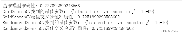

LightGBM

from lightgbm import LGBMClassifier
from sklearn.metrics import accuracy_score, classification_reportgbm = LGBMClassifier(learning_rate=0.02,n_estimators=100,max_depth=100)
# 训练模型
gbm.fit(X_train, y_train)# 进行预测
predictions = gbm.predict(X_test)# 评估模型
accuracy = accuracy_score(y_test, predictions)
report = classification_report(y_test, predictions)print(f"模型准确率：{accuracy}")
print(f"分类报告：\n{report}")

MLP-pytorch版

import torch
import torch.nn as nn
import torch.optim as optim
import numpy as np
import matplotlib.pyplot as plt# 假设 X_train、y_train、X_test、y_test 是 Pandas DataFrame
# 将 DataFrame 转换为 NumPy 数组
X_train_array = X_train.to_numpy().astype(np.float32)
y_train_array = y_train.to_numpy().astype(np.float32)
X_test_array = X_test.to_numpy().astype(np.float32)
y_test_array = y_test.to_numpy().astype(np.float32)# 转换数据为 PyTorch 张量
X_train_tensor = torch.from_numpy(X_train_array)
y_train_tensor = torch.from_numpy(y_train_array)
X_test_tensor = torch.from_numpy(X_test_array)
y_test_tensor = torch.from_numpy(y_test_array)# 定义简单的 MLP 模型
class MLP(nn.Module):def __init__(self):super(MLP, self).__init__()self.fc1 = nn.Linear(in_features=INPUT_SIZE, out_features=128)# 线性层self.relu = nn.ReLU()# 激活函数self.fc2 = nn.Linear(in_features=128, out_features=1)# 线性层self.sigmoid = nn.Sigmoid()# 激活函数def forward(self, x):x = self.relu(self.fc1(x))x = self.sigmoid(self.fc2(x))return x# 初始化模型、损失函数和优化器
INPUT_SIZE = X_train.shape[1]
mlp = MLP()
criterion = nn.BCELoss()
optimizer = optim.Adam(mlp.parameters(), lr=0.01)# 训练模型，并记录损失值
train_losses = []
val_losses = []
mlp.train()
for epoch in range(50):  # 迭代50次optimizer.zero_grad()outputs = mlp(X_train_tensor)loss = criterion(outputs, y_train_tensor.view(-1, 1))loss.backward()optimizer.step()train_losses.append(loss.item())mlp.eval()
with torch.no_grad():outputs_val = mlp(X_test_tensor)val_loss = criterion(outputs_val, y_test_tensor.view(-1, 1))val_losses.append(val_loss.item())# 计算预测准确率
accuracy = accuracy_score(y_test, predictions)
print(f"模型准确率：{accuracy}")

XGBoost-MLP-随机森林加权组合-效果最优

重新读取数据并转换编码和归一化操作

import pandas as pd
import numpy as np
import matplotlib.pyplot as plt
import seaborn as sns
from scipy import stats
from scipy.special import boxcox1p
import missingno as msno
import warnings
warnings.filterwarnings("ignore")%matplotlib inline
train = pd.read_csv('train.csv')
test = pd.read_csv('test_noLabel.csv')
train.shape,test.shape

from sklearn.preprocessing import LabelEncodercolumns_to_encode = ['Contract', 'Dependents', 'DeviceProtection', 'InternetService', 'MultipleLines', 'Partner', 'PaymentMethod', 'PhoneService', 'TVProgram', 'gender']for column in columns_to_encode:label_encoder = LabelEncoder()# 合并训练集和测试集的数据进行拟合combined_data = pd.concat([train[column], test[column]])label_encoder.fit(combined_data)# 对训练集进行映射train[column] = label_encoder.transform(train[column])test[column] = label_encoder.transform(test[column])# 初始化LabelEncoder并对训练集中的标签列进行映射
label_encoder = LabelEncoder()
train['Label'] = label_encoder.fit_transform(train['Label'])

train.drop('ID', axis=1, inplace=True)
test.drop('ID', axis=1, inplace=True)
# 提取特征数据与目标数据
train_noLabel = train.iloc[:, :-1]  # 选择除最后一列外的所有列作为特征
y= train['Label']  # 标签列

# 把train数据划分成训练数据0.8跟测试数据0.2，
from sklearn.model_selection import train_test_split
x_train,x_test,y_train,y_test = train_test_split(train_noLabel,y,test_size=0.2)print("x_train shape:", x_train.shape, "x_test shape:", x_test.shape, "y_train shape:", y_train.shape, "y_test shape:", y_test.shape)from sklearn.preprocessing import MinMaxScaler# 需要归一化的列
columns_to_normalize = ['MonthlyCharges', 'TotalCharges', 'tenure']# 初始化MinMaxScaler
scaler = MinMaxScaler()# 对训练集中的指定列进行归一化
x_train[columns_to_normalize] = scaler.fit_transform(x_train[columns_to_normalize])# 对测试集中的相同列进行归一化
x_test[columns_to_normalize] = scaler.transform(x_test[columns_to_normalize])
test[columns_to_normalize] = scaler.transform(test[columns_to_normalize])

from xgboost import XGBClassifier
from sklearn.neural_network import MLPClassifier
from sklearn.ensemble import RandomForestClassifier
from sklearn.model_selection import train_test_split, RandomizedSearchCV
from scipy.stats import randint, uniform
from sklearn.metrics import accuracy_score, classification_report
from bayes_opt import BayesianOptimization# XGBoost 超参数调优
def xgb_cv(learning_rate, n_estimators, max_depth, min_child_weight, subsample, gamma):xgb_model = XGBClassifier(learning_rate=learning_rate,n_estimators=int(n_estimators),max_depth=int(max_depth),min_child_weight=int(min_child_weight),subsample=subsample,gamma=gamma,random_state=42)xgb_model.fit(x_train, y_train)predictions = xgb_model.predict(x_test)accuracy = accuracy_score(y_test, predictions)return accuracyparam_bounds_xgb = {'learning_rate': (0.001, 0.01),'n_estimators': (50, 300),'max_depth': (3, 20),'min_child_weight': (1, 30),'subsample': (0.1, 1),'gamma': (0, 5)
}xgb_bayesian = BayesianOptimization(f=xgb_cv, pbounds=param_bounds_xgb, random_state=42)
xgb_bayesian.maximize(init_points=5, n_iter=100)
best_params_xgb = xgb_bayesian.max['params']
best_xgb_model = XGBClassifier(learning_rate=best_params_xgb['learning_rate'],n_estimators=int(best_params_xgb['n_estimators']),max_depth=int(best_params_xgb['max_depth']),min_child_weight=int(best_params_xgb['min_child_weight']),subsample=best_params_xgb['subsample'],gamma=best_params_xgb['gamma'],random_state=42
)
best_xgb_model.fit(x_train, y_train)# MLP 超参数调优
mlp = MLPClassifier(random_state=42)
param_dist_mlp = {'hidden_layer_sizes': [(64,), (128,), (256,)],'activation': ['relu', 'tanh', 'logistic'],'max_iter': randint(50, 200),'learning_rate_init': uniform(0.001, 0.1),
}
random_search_mlp = RandomizedSearchCV(mlp, param_distributions=param_dist_mlp, n_iter=10, cv=3, scoring='accuracy', random_state=42)
random_search_mlp.fit(x_train, y_train)
best_params_mlp = random_search_mlp.best_params_
best_model_mlp = random_search_mlp.best_estimator_# 随机森林超参数调优
base_model_rf = RandomForestClassifier()
param_dist_rf = {'n_estimators': randint(10, 200),'max_features': ['auto', 'sqrt', 'log2', None],'max_depth': [None, 10, 20, 30, 40, 50],'min_samples_split': randint(2, 20),'min_samples_leaf': randint(1, 20),'bootstrap': [True, False],'random_state': [42],
}
random_search_rf = RandomizedSearchCV(base_model_rf,param_distributions=param_dist_rf,n_iter=10,cv=5,scoring='accuracy',random_state=42,n_jobs=-1
)
random_search_rf.fit(x_train, y_train)
best_params_rf = random_search_rf.best_params_
best_model_rf = random_search_rf.best_estimator_# 组合模型并加权
predictions_xgb = best_xgb_model.predict(x_test)
predictions_mlp = best_model_mlp.predict(x_test)
predictions_rf = best_model_rf.predict(x_test)# 组合模型结果并加权
weighted_predictions = (0.4 * predictions_xgb) + (0.3 * predictions_mlp) + (0.3 * predictions_rf)# 将连续值转换为二元分类值
threshold = 0.5
binary_predictions = [1 if pred > threshold else 0 for pred in weighted_predictions]# 计算二元分类准确率
accuracy_binary = accuracy_score(y_test, binary_predictions)
report_binary = classification_report(y_test, binary_predictions)print(f"模型准确率: {accuracy_binary}")
print(f"二元分类模型准确率: {accuracy_binary}")
print(f"分类报告:\n{report_binary}")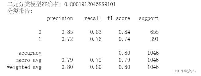

对测试数据进行分类预测并提交网站

# 进行预测# 组合模型并加权
predictions_xgb = best_xgb_model.predict(test)
predictions_mlp = best_model_mlp.predict(test)
predictions_rf = best_model_rf.predict(test)# 组合模型结果并加权
weighted_predictions = (0.4 * predictions_xgb) + (0.3 * predictions_mlp) + (0.3 * predictions_rf)# 将连续值转换为二元分类值
threshold = 0.5
binary_predictions = [1 if pred > threshold else 0 for pred in weighted_predictions]submit_example = pd.read_csv('submit_example.csv')  # 读取提交示例文件
# 替换 submit_example 的 Label 列
submit_example['Label'] = binary_predictions  # 将预测结果填入 submit_example 的 Label 列
submit_example['Label'] = label_encoder.inverse_transform(submit_example['Label'])  # 对 Label 进行反向转换
# 将结果写入 CSV 文件
submit_example.to_csv('zuhe_predict.csv', index=False)  # 将结果保存为 CSV 文件，不保存索引列