week43 aGNN

摘要

本周阅读了题为Contaminant Transport Modeling and Source AttributionWith Attention‐Based Graph Neural Network的论文。该文提出了 aGNN，它是一种新颖的基于注意力的图神经建模框架，它结合了图卷积网络（GCN）、注意力机制和嵌入层来模拟地下水中的污染物传输过程系统。 GCN 通过传递节点和边的消息来提取图信息，以有效地学习空间模式。在这项研究中，将其应用扩展到学习地下水流和溶质输送问题的多个过程。此外，还采用新的坐标嵌入方法在尚未研究的不受监控的污染位置进行归纳学习。注意力机制是 Transformer 网络中的关键组成部分，擅长顺序分析。嵌入层是潜在空间学习机制，代表时空过程中的高维性。

Abstract

This week’s weekly newspaper decodes the paper entitled Contaminant Transport Modeling and Source AttributionWith Attention‐Based Graph Neural Network. This paper proposes aGNN, a novel attention-based graph neural modeling framework, which combines graph convolutional networks (GCNs), attention mechanisms, and embedding layers to model contaminant transport processes in groundwater. GCNs extract graph information by passing messages from nodes and edges to learn spatial patterns efficiently. In this study, its application was extended to the study of multiple processes for groundwater flow and solute transport problems. In addition, a new coordinate embedding method was used to perform inductive learning at unmonitored contaminated locations that had not yet been studied. Attention mechanisms are a key component in the Transformer network and excel at sequential analysis. The embedding layer is a latent spatial learning mechanism, which represents the high-dimensionality of spatiotemporal processes.

1. 题目

标题：Contaminant Transport Modeling and Source AttributionWith Attention‐Based Graph Neural Network

作者：Min Pang1,2,3, Erhu Du2,3 , and Chunmiao Zheng3,4,5

发布：Water Resources Research Volume 60, Issue 6 e2023WR035278

链接：https://doi.org/10.1029/2023WR035278

2. Abstract

该文引入了一种新的基于注意力的图神经网络（aGNN），用于利用有限的监测数据对污染物传输进行建模，并量化污染物源（驱动因素）与其传播（结果）之间的因果关系。在涉及异质含水层中不同监测网络的五个综合案例研究中，aGNN 在多步预测（即传导学习）中表现优于基于 LSTM（长期短期记忆）和 CNN（卷积神经网络）的方法。它还证明了在推断未监测站点的观察（即归纳学习）方面的高水平适用性。此外，基于 aGNN 的解释性分析量化了每个污染物源的影响，并已通过基于物理的模型进行了验证，结果一致，R2 值超过 92%。 aGNN 的主要优点是它不仅在多场景评估中具有高水平的预测能力，而且还大大降低了计算成本。总体而言，这项研究表明，aGNN 对于地下污染物传输的高度非线性时空学习来说是高效且稳健的，并为涉及污染物源归因的地下水管理提供了一种有前景的工具。

3. 网络架构

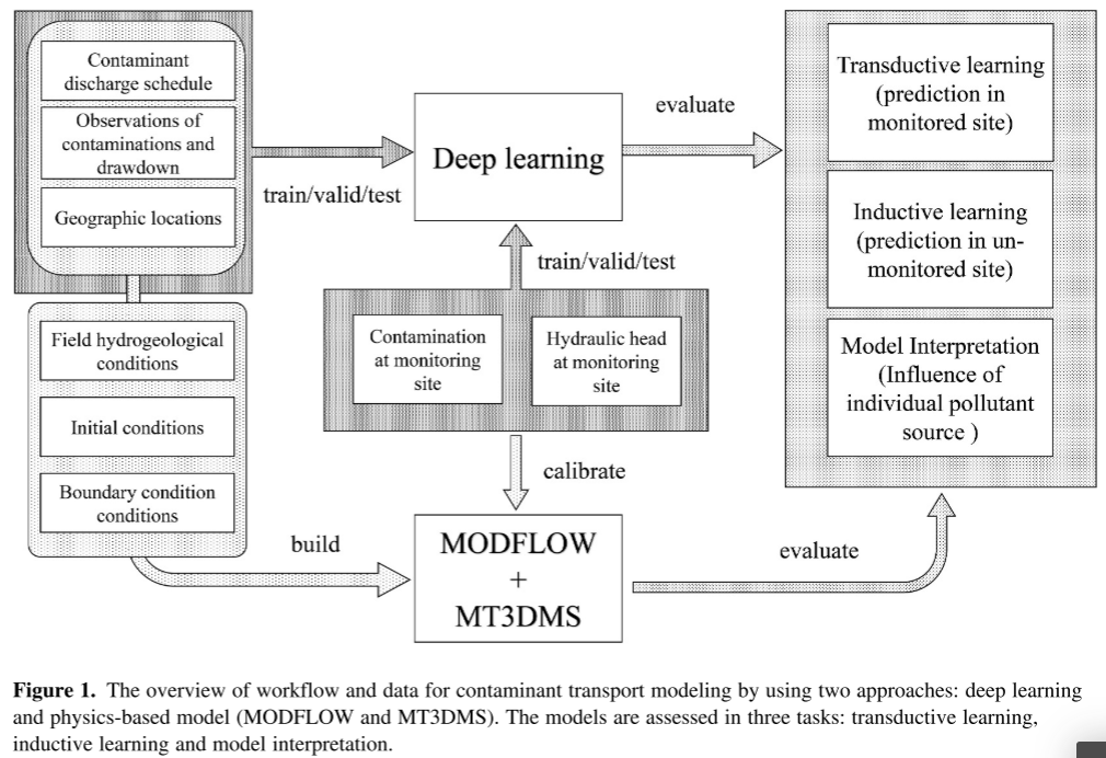
图 1 显示了两种方法（即深度学习方法和基于物理的模型）的工作流程，用于对地下水质量时空变化进行建模，以响应多个来源的污染物排放。

DL的输入数据包括排水表、污染物释放表、污染浓度和地下水位下降的观测数据。基于物理的模型提供了地面真实结果，可用于评估深度学习模型的性能（两个基准深度学习模型的详细信息，扩散卷积循环神经网络（DCRNN）和卷积长短期记忆（ConvLSTM）

使用 Shapley 值法进行模型解释来研究单个污染源的影响。深度学习模型的事后解释评估应用模型后每个源在关键位置的影响。

3.1 aGNN

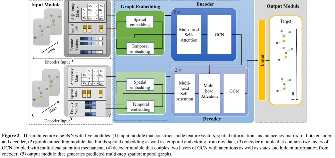
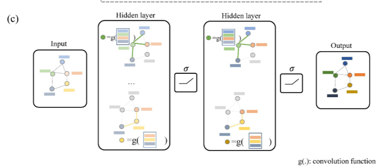
图 2 展示了 aGNN 的架构，它建立在编码器-解码器框架之上

aGNN 由五个模块组成：输入模块、图嵌入模块、编码器模块、解码器模块和输出模块。

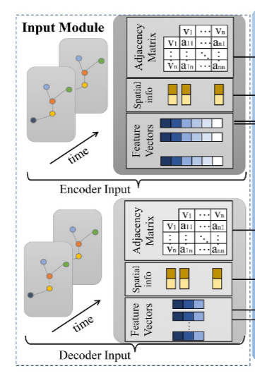
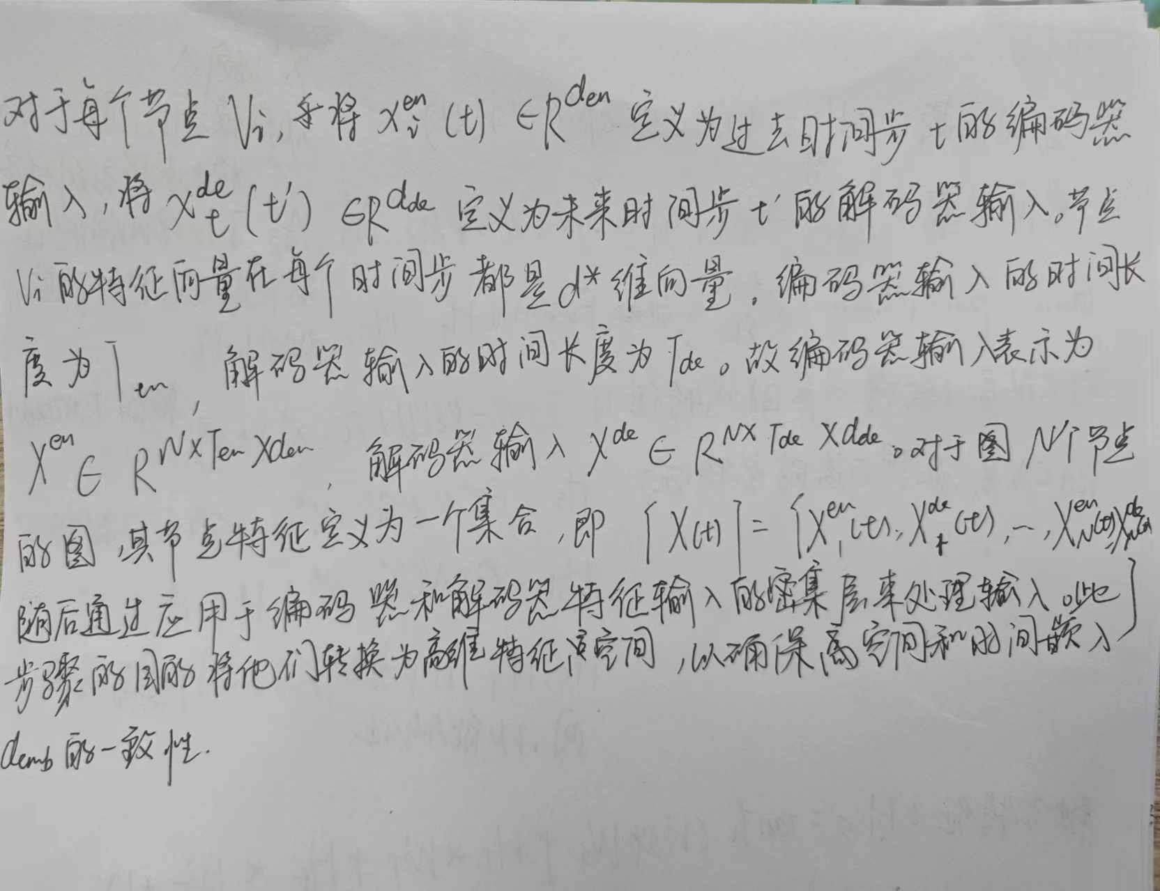
• 输入模块包含两个组件，即编码器输入和解码器输入，两者都呈现在时空图中。
• 对于这些高维输入，图嵌入模块结合了空间嵌入和时间嵌入，将原始输入转换为特征表示，该特征表示集成了来自补给计划、流动动力学和污染物传播的线索。
• 获得的表示被输入到编码器和解码器模块中以提取它们的相互关系。编码器模块和解码器模块都包含两层具有注意机制的图卷积网络

该网络的优点是

1. 注意力机制通过动态关注输入中最相关的部分来灵活地学习相互关系
2. GCN 有利于提取图的拓扑连接。解码器模块最后一层的输出进入输出模块，该模块生成目标序列预测作为诱发的污染物在空间和时间上的移动。

3.1.1 输入与输出模块

图的结构由节点 Vs 和边 Es 的集合组成（即 G = (V, E, A)）。在本研究中，节点集合V代表观测站点，节点Vi的节点表示xi可以是存储所有观测值的向量。 E 是连接两个节点 (Vi, Vj) 的边。 N × N 维的邻接矩阵（A）表示每两个节点之间的依赖关系，从而描述了图的拓扑结构。

为了建立图结构，对无向图使用加权邻接矩阵。如果存在连接节点 i 和节点 j 的边，则为邻接矩阵中的每个条目 (i, j) 分配一个非零权重；否则，它被设置为0。每个条目的权重由节点i和节点j之间的距离确定。

输出是多步预测，以时空图 (Y) 的形式呈现。这些预测涵盖所有节点，每个节点都有一个或多个目标。因此，每个节点 Vi 中的输出 $y_i(t)$ 可以是时间步 t 处的多维向量。总的来说，节点 Vi 的输出表示为 $Y_i(t)=[y_i(t+1),y_i(t+2),\dots ,y_i(t+Tde)]$，Tde 是预测范围，$Y(t)=Y_1(t),Y_2(t),\dots ,Y_N(t)$​ 表示快照时的输出图。

3.1.2 嵌入层

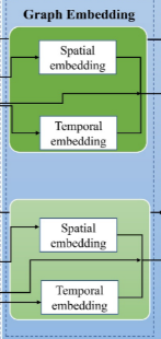
在 aGNN 中，开发并合并了一个嵌入模块来编码空间图中的空间异质性和时间序列中的顺序信息。空间异质性嵌入适用于地理坐标，并由径向基网络层构建。时间顺序信息建立在位置嵌入的基础上，在其应用中表现出与注意力机制相结合的协同效应。

基于接近度的邻接矩阵可能不足以描述隐式空间依赖性。此外，普通 GCN 缺乏将空间坐标信息转换为潜在空间的层，这使得它们在表示隐式空间依赖关系方面信息较少。

首先制定空间坐标矩阵$C\in R^{N\times 2}$，它由所有节点c1，…cN的地理坐标（即经度和纬度）组成。然后，将空间异质性嵌入定义为 $SE=\phi (F(C,l{o}_{max},l{a}_{max}),{\theta }_{sh})$​，其中 F 是从经度和纬度中提取信息的特征函数

函数 φ 是一个 RBN 网络，它将空间特征映射到维度为 $d_{emb}$ 的嵌入空间（即 φ : R2→ Rdemb ）。 ρ 是二次 RBF 函数。 φ被实现为具有可学习参数的用于空间异质性编码的全连接神经网络

$N_{ctr}$ 是中心数，定义为本研究中的节点数（即 $N_{ctr}=N$）。
$$\varphi (c_x)=\sum _{i=1}^{N_{ctr}}{a}_i\rho (||c_x-c_i^{ctr}||)$$
给定时间序列$S=(s_0,s_1,\dots ,s_T)$，时间嵌入层形成有限维表示来指示 $s_i$ 在序列 S 中的位置

研究中的时间嵌入是正弦变换到时间顺序的串联，形成矩阵 $TE\in RT\times d_{emb}$ ，其中 T 和 demb 分别是时间长度和向量维度。

TE由公式2和公式3设计，其中2d和2d+1分别表示偶数和奇数维度，t是时间序列中的时间位置。时间嵌入的维度为$d_{emb}\times T$。
$$T{E}_{(t,2d)}=sin(\frac{t}{10000^{\frac{2d}{d_{emb}}}})\text{\hspace{1em}(2)}$$

$$T{E}_{(t,2d+1)}=cos(\frac{t}{10000^{frac2d+1d_{emb}}})\text{\hspace{1em}(3)}$$

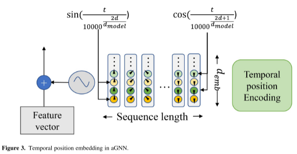
如图3所示，时间嵌入中的每个元素结合了时间顺序位置和特征空间的信息。

3.1.3编码器解码器模块：带有多头注意力层的GCN

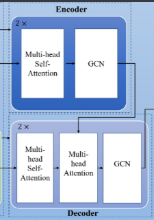
编码器和解码器都由多层构建块组成，包括多头自注意力（MSA）、GCN 和多头注意力（MAT）块。 MSA 对时间序列本身的动态相关性进行建模，GCN 尝试捕获监测站观测值之间的空间相关依赖性，而 MAT 将信息从编码器传输到解码器。

注意力机制

在注意力机制中，输入数据被定义为三种不同的类型：查询（Q）、键（K）和值（V）。这个想法是将一个 Q 和一组 K-V 对映射到一个输出，使得输出表示 V 的加权和。
$$Attention(Q,K,V)=softmax(\frac{Q{K}^T}{{\sqrt{d}}_{model}})V$$

多头自注意力机制

在 MAT 中，Q、K 和 V 通过不同的学习线性变换（公式 5 和公式 6）投影 h 次。
$$multihead(Q,K,V)=concat(hea{d}_1,\dots ,hea{d}_h)W^m\text{\hspace{1em}(5)}$$

$$hea{d}_i=Attention(X_q,W_i^Q,X_k{W}_i^K,X_V{W}_i^V)\text{\hspace{1em}(6)}$$

GCN

GCN 的主要思想是构建一个消息传递网络，其中信息沿着图中的相邻节点传播。

从节点角度来看，GCN 首先聚合相邻节点的特征表示，并通过线性变换和非线性激活更新每个节点的状态。所有节点都通过图中的链接演化，并在 GCN 的一层或多层之间进行转换，从而允许学习图结构数据集之间的复杂依赖关系。类似于地统计插值方法，GCN 可以通过归纳学习将提取的依赖关系表示推广到看不见的节点。

对于输入矩阵 $Z\in R^{N\times d_{emb}}$ ，GCN 通过添加自循环的邻接矩阵（A）聚合节点的邻近特征及其特征（即 $\tilde{A}=A+I$），信息传播为表示为 ${\tilde{D}}^{\frac{-1}{2}}\tilde{A}{\tilde{D}}^{\frac{-1}{2}}Z$，利用图拉普拉斯矩阵来收集邻近信息。

随后应用线性投影和非线性变换，如方程 7 所示，其中 σ 是非线性激活函数，$W\in R^{d_{emb}\times d_{emb}}$​ 是可学习的线性化参数。
$$GCN(Z)=\sigma ({\tilde{D}}^{\frac{-1}{2}}\tilde{A}{\tilde{D}}^{\frac{-1}{2}}ZW)\text{\hspace{1em}(7)}$$

3.2 可释性模型：SHAP

Shapley价值法量化了合作过程中每个参与者的贡献，当他们的行为导致联合结果时。它可用于衡量深度学习方法中的特征重要性。通过 SHAP 评估每个污染物源的影响。

在具有 N 个污染源/点的字段中，令 SN 表示 N 点的子集，$f_{i.j}(SN)$ 表示当仅子集 SN 中的污染物源污染地下水时，给定位置单元格 (i,j) 处诱发的污染物浓度。特定点 d (d = 1,…, n) 的 Shapley 值 ${\Phi }_{i,j}$​可由公式 8 表示。
Φ i , j = ∑ S N ⊆ N ∣ S N ∣ ! ( n − ∣ S N ∣ − 1 ) ! N ! [ f i . j S N ∪ { d } − f i . j ( S N ) ] (8) \Phi_{i,j}=\sum_{SN\subseteq N}\frac{|SN|!(n-|SN|-1)!}{N!}[f_{i.j}SN\cup \{d\}-f_{i.j}(SN)] \tag{8} Φi,j​=SN⊆N∑​N!∣SN∣!(n−∣SN∣−1)!​[fi.j​SN∪{d}−fi.j​(SN)](8)

4. 文献解读

4.1 Introduction

该文提出了 aGNN，它是一种新颖的基于注意力的图神经建模框架，它结合了图卷积网络（GCN）、注意力机制和嵌入层来模拟地下水中的污染物传输过程系统。 GCN 通过传递节点和边的消息来提取图信息，以有效地学习空间模式。在这项研究中，将其应用扩展到学习地下水流和溶质输送问题的多个过程。此外，还采用新的坐标嵌入方法在尚未研究的不受监控的污染位置进行归纳学习。注意力机制是 Transformer 网络中的关键组成部分，擅长顺序分析。嵌入层是潜在空间学习机制，代表时空过程中的高维性。

4.2 创新点

该文的主要贡献有四个方面：

1. 研究了 aGNN 在涉及污染物传输建模的多过程中的性能。基于 GNN、CNN、LSTM 的方法适用于多步超前空间预测的相同端到端学习任务，以深入了解每个模型的性能。
2. 根据数据的可用性和含水层的异质性，评估 aGNN 通过归纳学习将从监测数据中学到的知识转移到未监测站点的能力。
3. 采用了一种可解释的人工智能技术，即沙普利值（Shapley value），它起源于合作博弈论的概念。在本研究中，Shapley值代表多源排放情况下的污染物源归因。
4. 评估了使用 aGNN 与使用基于物理的模型相比的时间效率。从三个不同的方面证明，基于注意力的图模型是污染建模的一种前瞻性工具，可以为地下水污染管理的政策制定者提供信息。

4.3 实验过程

4.3.1 实验区域以及场景设置

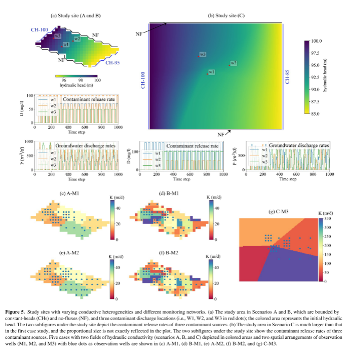
在这项研究中，设计了两个以无承压含水层为特色的综合研究地点，用于方法开发和验证。第一个研究点面积为 497,500 $m^2$​，如图 5a 所示，在 MODFLOW 中离散化为 30 列和 15 行（每个单元为 50 m x 50 m）。水文边界被建模为无通量边界的两侧和恒定水头的两侧（分别为100和95 m）（图5a），自然水力梯度驱动地下水流。水文地质设置为：比产率为0.3，比库为0.0001 1/m，孔隙度为0.3。为了研究水力传导率 (HC) 异质性对污染物迁移模型的影响，本研究考虑了两个水力传导率领域：

（a）场景 A：由五个不同区域组成的领域，水力传导率从 15 到 35 m/天不等（图 5c 和 5e）和

（b）场景 B：水力传导率更加多样化的区域，范围从 0 到 50 m/天（图 5d 和 5f）。

在 MT3DMS 中，污染物传输采用整个研究区域 30 m 的均匀纵向分散度进行建模。研究域内的污染活动涉及三口注入井间歇性地将污染水排入地下水含水层，分别表示为位于上游的W3和位于相对下游的W1和W2（图5a）。三口井的定期排放时间表和污染物释放率如图 5a 所示，该图描绘了 2,100 天的整个观测周期的部分序列。地下水流和污染物迁移模型都是瞬态的，有 2,100 个时间步长，每个时间步长为 1 d。

第二个研究地点（场景 C）占地 180 平方公里，大约是第一个研究地点的 360 倍（图 5b）。它在 MODFLOW 中被离散化为 120 列和 150 行，每个单元尺寸为 100 m x 100 m。水文地质边界采用两侧作为无通量边界和两侧作为常水头边界（具体来说，分别为 100 和 85 m）进行建模。水力传导率异质性范围很大，由四个不同的区域表示，水力传导率从 30 到 350 m/天不等（图 5g）。其余的水文地质环境与第一个研究地点的水文地质环境一致。同样，污染活动涉及三个注入井（即 W1、W2 和 W3）按照定期排放时间表和特定的污染物释放速率间歇性地将污染水排放到地下水含水层中，如图 5a 所示。

4.3.2 数据预处理

污染物迁移数据集是通过 MODFLOW 和 MT3DMS 模拟这五种情况生成的。所有数据样本中，80%用于训练DL模型，其余20%用于性能评估。所有深度学习模型均通过批量优化对大型时空数据集进行训练，批量大小为 16，历时 400 个周期，输出是 GD 和 CC 在观测位置的预测，时间范围为 50 个时间步长。

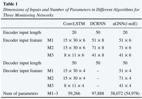
深度学习模型包括 DCRNN、aGNN、aGNN-noE（即没有嵌入模块的 aGNN 变体）和 ConvLSTM。所有算法都使用编码器-解码器框架，但输入的设计存在差异。表 1 总结了所有四种算法的输入维度。

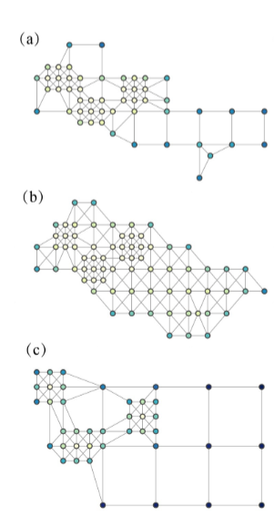
图 6a-6c 描述了三个监控系统的配置，每个监控系统对应一个场景。

归纳学习中使用的图形结构如图 6d-6f 所示，代表案例 M1、M2 和 M3 的预测区域。

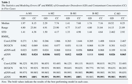
表 2 概述了建模目标在整个数据集中的统计特征，分为 80/20 的训练和测试分组。此外，结果还展示了 aGNN 在五个不同案例的测试数据上的性能

表 2 还表明，含水层非均质性对 GD 引起的变化产生影响，但程度比 CC 中的影响小得多，这尤其体现在情景 A 和 B 之间的不同值范围中。

由于含水层设置和提供的数据对预测任务产生不同程度的影响，我们使用这些案例来评估四个模型的性能，包括 aGNN 和三个基准模型，即 DCGCN、ConvLSTM 和 aGNN-noE。使用两种度量，即 $R_a^2$ 和 $RMS{E}_a$，来分析跨空间 S 和时间 T 的场的整体时空预测 ($x_{s,t}$)。

GNN 在几乎所有五种情况下都获得了最低的$RMS{E}_a$和最高的 $R_a^2$。表2表明与其他算法相比，aGNN 在对不均匀分布的监测系统中的污染物传输进行建模方面具有优越的性能。

CC是模拟污CC染物传输的主要目标。进一步分析了各种模型在空间和时间预测中的特征，使用两种度量作为 RMSE，它描述了建模精度的空间变化，而 $RMS{E}_t$​则说明了不同的时间变化。预测精度。

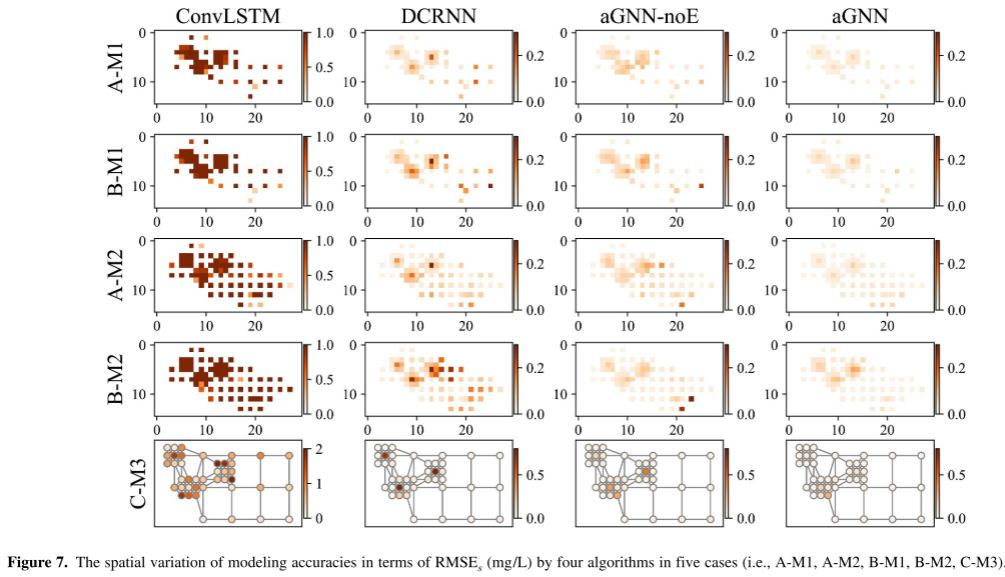
图 7 中的 RMSE 字段展示了四个模型的预测误差。如图 7 所示，aGNN-noE 和 aGNN 均优于 DCRNN，且该区域的 RMSE 变化相对较小，这表明基于注意力的图卷积网络优于扩散卷积图网络

5. 结论

在该研究中，证明基于 GNN 的模型非常适合该方面的挑战。节点和边是图结构数据中的两个重要特征，使得图网络中的信息传输成为可能，这类似于基于物理的地下水流和溶质运移运动，并且可以推广到任何不规则结构的水质监测网络。这项研究的主要贡献是在 aGNN 中融入了三个重要的构建模块，即注意力机制和时空嵌入层以及学习污染物传输中响应人为来源的高度非线性时空依赖性的 GCN 层。这三个构建模块通过在污染物传输的基于物理的图结构中采用动态权重分配、先验特征转换和信息传输来提高时空学习的准确性。

在实验中，aGNN 的 $R^2$ 值高达 99%，展示了集成注意力机制和嵌入层的高水平预测能力。我们的结果还说明了使用 aGNN 通过图学习进行知识泛化，根据受监控位置提供的数据推断出不受监控位置的观测结果的潜力。

尽管数据有限，aGNN 可以有效地利用现有信息来推断污染物运动的时空变化，即使是在异质性较高的含水层中，或在监测井有限的大型地点。然而，值得注意的是，可用数据量对于精确推理至关重要，因为更大的数据量可以提高建模精度，并且可以提高可迁移性和归纳分析的准确性。可以探索进一步的研究，例如优化监控网络系统，以提高监控系统的效率。

6.代码复现

1. 实验结果

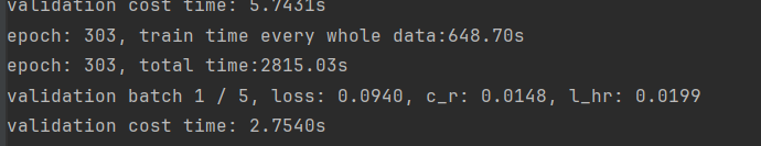
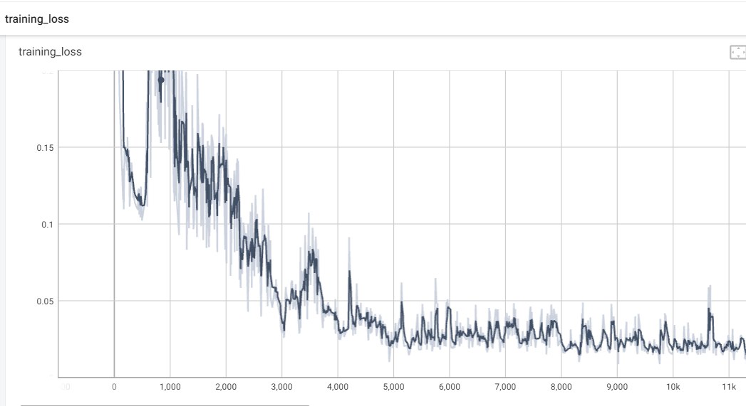
训练epoch300，调参epoch3，训练结果如下

训练集损失变化如下

验证集损失变化如下

2. 模型代码

import torch
import torch.nn as nn
import torch.nn.functional as F
import copy
import math
import numpy as np
from utils_dpl3_contam import norm_Adjclass RBF(nn.Module):"""Transforms incoming data using a given radial basis function:u_{i} = rbf(||x - c_{i}|| / s_{i})Arguments:in_features: size of each input sampleout_features: size of each output sampleShape:- Input: (N, in_features) where N is an arbitrary batch size- Output: (N, out_features) where N is an arbitrary batch sizeAttributes:centres: the learnable centres of shape (out_features, in_features).The values are initialised from a standard normal distribution.Normalising inputs to have mean 0 and standard deviation 1 isrecommended.log_sigmas: logarithm of the learnable scaling factors of shape (out_features).basis_func: the radial basis function used to transform the scaleddistances."""def __init__(self, in_features, out_features, num_vertice,basis_func):super(RBF, self).__init__()self.in_features = in_featuresself.out_features = out_featuresself.centres1 = nn.Parameter(torch.Tensor(num_vertice, self.in_features))  # (out_features, in_features)self.alpha = nn.Parameter(torch.Tensor(num_vertice,out_features))self.log_sigmas = nn.Parameter(torch.Tensor(out_features))self.basis_func = basis_funcself.reset_parameters()# self.alpha1 = nn.Parameter(torch.Tensor(num_vertice, self.out_features))def reset_parameters(self):nn.init.normal_(self.centres1, 0, 1)nn.init.constant_(self.log_sigmas, 0)def forward(self, input):size1= (input.size(0), input.size(0), self.in_features)x1 = input.unsqueeze(1).expand(size1)c1 = self.centres1.unsqueeze(0).expand(size1)distances1 = torch.matmul((x1 - c1).pow(2).sum(-1).pow(0.5),self.alpha) / torch.exp(self.log_sigmas).unsqueeze(0)return self.basis_func(distances1) #distances1# RBFsdef gaussian(alpha):phi = torch.exp(-1 * alpha.pow(2))return phidef linear(alpha):phi = alphareturn phidef quadratic(alpha):phi = alpha.pow(2)return phidef inverse_quadratic(alpha):phi = torch.ones_like(alpha) / (torch.ones_like(alpha) + alpha.pow(2))return phidef multiquadric(alpha):phi = (torch.ones_like(alpha) + alpha.pow(2)).pow(0.5)return phidef inverse_multiquadric(alpha):phi = torch.ones_like(alpha) / (torch.ones_like(alpha) + alpha.pow(2)).pow(0.5)return phidef spline(alpha):phi = (alpha.pow(2) * torch.log(alpha + torch.ones_like(alpha)))return phidef poisson_one(alpha):phi = (alpha - torch.ones_like(alpha)) * torch.exp(-alpha)return phidef poisson_two(alpha):phi = ((alpha - 2 * torch.ones_like(alpha)) / 2 * torch.ones_like(alpha)) \* alpha * torch.exp(-alpha)return phidef matern32(alpha):phi = (torch.ones_like(alpha) + 3 ** 0.5 * alpha) * torch.exp(-3 ** 0.5 * alpha)return phidef matern52(alpha):phi = (torch.ones_like(alpha) + 5 ** 0.5 * alpha + (5 / 3) \* alpha.pow(2)) * torch.exp(-5 ** 0.5 * alpha)return phidef basis_func_dict():"""A helper function that returns a dictionary containing each RBF"""bases = {'gaussian': gaussian,'linear': linear,'quadratic': quadratic,'inverse quadratic': inverse_quadratic,'multiquadric': multiquadric,'inverse multiquadric': inverse_multiquadric,'spline': spline,'poisson one': poisson_one,'poisson two': poisson_two,'matern32': matern32,'matern52': matern52}return bases
###############################################################################################################def clones(module, N):'''Produce N identical layers.:param module: nn.Module:param N: int:return: torch.nn.ModuleList'''return nn.ModuleList([copy.deepcopy(module) for _ in range(N)])def subsequent_mask(size):'''mask out subsequent positions.:param size: int:return: (1, size, size)'''attn_shape = (1, size, size)subsequent_mask = np.triu(np.ones(attn_shape), k=1).astype('uint8')return torch.from_numpy(subsequent_mask) == 0   # 1 means reachable; 0 means unreachableclass spatialGCN(nn.Module):def __init__(self, sym_norm_Adj_matrix, in_channels, out_channels):super(spatialGCN, self).__init__()self.sym_norm_Adj_matrix = sym_norm_Adj_matrix  # (N, N)self.in_channels = in_channelsself.out_channels = out_channelsself.Theta = nn.Linear(in_channels, out_channels, bias=False)def forward(self, x):'''spatial graph convolution operation:param x: (batch_size, N, T, F_in):return: (batch_size, N, T, F_out)'''batch_size, num_of_vertices, num_of_timesteps, in_channels = x.shapex = x.permute(0, 2, 1, 3).reshape((-1, num_of_vertices, in_channels))  # (b*t,n,f_in)return F.relu(self.Theta(torch.matmul(self.sym_norm_Adj_matrix, x)).reshape((batch_size, num_of_timesteps, num_of_vertices, self.out_channels)).transpose(1, 2))class GCN(nn.Module):def __init__(self, sym_norm_Adj_matrix, in_channels, out_channels):super(GCN, self).__init__()self.sym_norm_Adj_matrix = sym_norm_Adj_matrix  # (N, N)self.in_channels = in_channelsself.out_channels = out_channelsself.Theta = nn.Linear(in_channels, out_channels, bias=False)def forward(self, x):'''spatial graph convolution operation:param x: (batch_size, N, F_in):return: (batch_size, N, F_out)'''return F.relu(self.Theta(torch.matmul(self.sym_norm_Adj_matrix, x)))  # (N,N)(b,N,in)->(b,N,in)->(b,N,out)class Spatial_Attention_layer(nn.Module):'''compute spatial attention scores'''def __init__(self, dropout=.0):super(Spatial_Attention_layer, self).__init__()self.dropout = nn.Dropout(p=dropout)def forward(self, x):''':param x: (batch_size, N, T, F_in):return: (batch_size, T, N, N)'''batch_size, num_of_vertices, num_of_timesteps, in_channels = x.shapex = x.permute(0, 2, 1, 3).reshape((-1, num_of_vertices, in_channels))  # (b*t,n,f_in)score = torch.matmul(x, x.transpose(1, 2)) / math.sqrt(in_channels)  # (b*t, N, F_in)(b*t, F_in, N)=(b*t, N, N)score = self.dropout(F.softmax(score, dim=-1))  # the sum of each row is 1; (b*t, N, N)return score.reshape((batch_size, num_of_timesteps, num_of_vertices, num_of_vertices))class spatialAttentionGCN(nn.Module):def __init__(self, sym_norm_Adj_matrix, in_channels, out_channels, dropout=.0):super(spatialAttentionGCN, self).__init__()self.sym_norm_Adj_matrix = sym_norm_Adj_matrix  # (N, N)self.in_channels = in_channelsself.out_channels = out_channelsself.Theta = nn.Linear(in_channels, out_channels, bias=False)self.SAt = Spatial_Attention_layer(dropout=dropout)def forward(self, x):'''spatial graph convolution operation:param x: (batch_size, N, T, F_in):return: (batch_size, N, T, F_out)'''batch_size, num_of_vertices, num_of_timesteps, in_channels = x.shapespatial_attention = self.SAt(x)  # (batch, T, N, N)x = x.permute(0, 2, 1, 3).reshape((-1, num_of_vertices, in_channels))  # (b*t,n,f_in)spatial_attention = spatial_attention.reshape((-1, num_of_vertices, num_of_vertices))  # (b*T, n, n)return F.relu(self.Theta(torch.matmul(self.sym_norm_Adj_matrix.mul(spatial_attention), x)).reshape((batch_size, num_of_timesteps, num_of_vertices, self.out_channels)).transpose(1, 2))# (b*t, n, f_in)->(b*t, n, f_out)->(b,t,n,f_out)->(b,n,t,f_out)class spatialAttentionScaledGCN(nn.Module):def __init__(self, sym_norm_Adj_matrix, in_channels, out_channels, dropout=.0):super(spatialAttentionScaledGCN, self).__init__()self.sym_norm_Adj_matrix = sym_norm_Adj_matrix  # (N, N)self.in_channels = in_channelsself.out_channels = out_channelsself.Theta = nn.Linear(in_channels, out_channels, bias=False)self.SAt = Spatial_Attention_layer(dropout=dropout)def forward(self, x):'''spatial graph convolution operation:param x: (batch_size, N, T, F_in):return: (batch_size, N, T, F_out)'''batch_size, num_of_vertices, num_of_timesteps, in_channels = x.shapespatial_attention = self.SAt(x) / math.sqrt(in_channels)  # scaled self attention: (batch, T, N, N)x = x.permute(0, 2, 1, 3).reshape((-1, num_of_vertices, in_channels))# (b, n, t, f)-permute->(b, t, n, f)->(b*t,n,f_in)spatial_attention = spatial_attention.reshape((-1, num_of_vertices, num_of_vertices))  # (b*T, n, n)return F.relu(self.Theta(torch.matmul(self.sym_norm_Adj_matrix.mul(spatial_attention), x)).reshape((batch_size, num_of_timesteps, num_of_vertices, self.out_channels)).transpose(1, 2))# (b*t, n, f_in)->(b*t, n, f_out)->(b,t,n,f_out)->(b,n,t,f_out)class SpatialPositionalEncoding_RBF(nn.Module):def __init__(self, d_model, logitudelatitudes,num_of_vertices, dropout, gcn=None, smooth_layer_num=0):super(SpatialPositionalEncoding_RBF, self).__init__()self.dropout = nn.Dropout(p=dropout)# self.embedding = torch.nn.Embedding(num_of_vertices, d_model)self.embedding = RBF(2, d_model, num_of_vertices,quadratic) # gaussin nn.Linear(4, d_model-4)self.logitudelatitudes = logitudelatitudesself.gcn_smooth_layers = Noneif (gcn is not None) and (smooth_layer_num > 0):self.gcn_smooth_layers = nn.ModuleList([gcn for _ in range(smooth_layer_num)])def forward(self, x,log1,lat1):''':param x: (batch_size, N, T, F_in):return: (batch_size, N, T, F_out)'''# x,log,lat,t= x[0],x[1],x[2],x[3]batch, num_of_vertices, timestamps, _ = x.shapex_indexs = torch.concat((torch.unsqueeze(log1.mean(0).mean(-1),-1),torch.unsqueeze(lat1.mean(0).mean(-1),-1)),-1)# (N,)x_ind = torch.concat((x_indexs[:, 0:1] ,x_indexs[:, 1:] ), axis=1)embed = self.embedding(x_ind.float()).unsqueeze(0)if self.gcn_smooth_layers is not None:for _, l in enumerate(self.gcn_smooth_layers):embed = l(embed)  # (1,N,d_model) -> (1,N,d_model)x = x + embed.unsqueeze(2)  # (B, N, T, d_model)+(1, N, 1, d_model)return self.dropout(x)class TemporalPositionalEncoding(nn.Module):def __init__(self, d_model, dropout, max_len, lookup_index=None):super(TemporalPositionalEncoding, self).__init__()self.dropout = nn.Dropout(p=dropout)self.lookup_index = lookup_indexself.max_len = max_len# computing the positional encodings once in log spacepe = torch.zeros(max_len, d_model)for pos in range(max_len):for i in range(0, d_model, 2):pe[pos, i] = math.sin(pos / (10000 ** ((2 * i)/d_model)))pe[pos, i+1] = math.cos(pos / (10000 ** ((2 * (i + 1)) / d_model)))pe = pe.unsqueeze(0).unsqueeze(0)  # (1, 1, T_max, d_model)self.register_buffer('pe', pe)# register_buffer:# Adds a persistent buffer to the module.# This is typically used to register a buffer that should not to be considered a model parameter.def forward(self, x,t):''':param x: (batch_size, N, T, F_in):return: (batch_size, N, T, F_out)'''if self.lookup_index is not None:x = x + self.pe[:, :, self.lookup_index, :]  # (batch_size, N, T, F_in) + (1,1,T,d_model)else:x = x + self.pe[:, :, :x.size(2), :]return self.dropout(x.detach())class SublayerConnection(nn.Module):'''A residual connection followed by a layer norm'''def __init__(self, size, dropout, residual_connection, use_LayerNorm):super(SublayerConnection, self).__init__()self.residual_connection = residual_connectionself.use_LayerNorm = use_LayerNormself.dropout = nn.Dropout(dropout)if self.use_LayerNorm:self.norm = nn.LayerNorm(size)def forward(self, x, sublayer):''':param x: (batch, N, T, d_model):param sublayer: nn.Module:return: (batch, N, T, d_model)'''if self.residual_connection and self.use_LayerNorm:return x + self.dropout(sublayer(self.norm(x)))if self.residual_connection and (not self.use_LayerNorm):return x + self.dropout(sublayer(x))if (not self.residual_connection) and self.use_LayerNorm:return self.dropout(sublayer(self.norm(x)))class PositionWiseGCNFeedForward(nn.Module):def __init__(self, gcn, dropout=.0):super(PositionWiseGCNFeedForward, self).__init__()self.gcn = gcnself.dropout = nn.Dropout(dropout)def forward(self, x):''':param x:  (B, N_nodes, T, F_in):return: (B, N, T, F_out)'''return self.dropout(F.relu(self.gcn(x)))def attention(query, key, value, mask=None, dropout=None):''':param query:  (batch, N, h, T1, d_k):param key: (batch, N, h, T2, d_k):param value: (batch, N, h, T2, d_k):param mask: (batch, 1, 1, T2, T2):param dropout::return: (batch, N, h, T1, d_k), (batch, N, h, T1, T2)'''d_k = query.size(-1)scores = torch.matmul(query, key.transpose(-2, -1)) / math.sqrt(d_k)  # scores: (batch, N, h, T1, T2)if mask is not None:scores = scores.masked_fill_(mask == 0, -1e9)  # -1e9 means attention scores=0p_attn = F.softmax(scores, dim=-1)if dropout is not None:p_attn = dropout(p_attn)# p_attn: (batch, N, h, T1, T2)return torch.matmul(p_attn, value), p_attn  # (batch, N, h, T1, d_k), (batch, N, h, T1, T2)class MultiHeadAttention(nn.Module):def __init__(self, nb_head, d_model, dropout=.0):super(MultiHeadAttention, self).__init__()assert d_model % nb_head == 0self.d_k = d_model // nb_headself.h = nb_headself.linears = clones(nn.Linear(d_model, d_model), 4)self.dropout = nn.Dropout(p=dropout)def forward(self, query, key, value, mask=None):''':param query: (batch, N, T, d_model):param key: (batch, N, T, d_model):param value: (batch, N, T, d_model):param mask: (batch, T, T):return: x: (batch, N, T, d_model)'''if mask is not None:mask = mask.unsqueeze(1).unsqueeze(1)  # (batch, 1, 1, T, T), same mask applied to all h heads.nbatches = query.size(0)N = query.size(1)# (batch, N, T, d_model) -linear-> (batch, N, T, d_model) -view-> (batch, N, T, h, d_k) -permute(2,3)-> (batch, N, h, T, d_k)query, key, value = [l(x).view(nbatches, N, -1, self.h, self.d_k).transpose(2, 3) for l, x inzip(self.linears, (query, key, value))]# apply attention on all the projected vectors in batchx, self.attn = attention(query, key, value, mask=mask, dropout=self.dropout)# x:(batch, N, h, T1, d_k)# attn:(batch, N, h, T1, T2)x = x.transpose(2, 3).contiguous()  # (batch, N, T1, h, d_k)x = x.view(nbatches, N, -1, self.h * self.d_k)  # (batch, N, T1, d_model)return self.linears[-1](x)class MultiHeadAttentionAwareTemporalContex_qc_kc(nn.Module):  # key causal; query causal;def __init__(self, nb_head, d_model, num_of_lags, points_per_lag, kernel_size=3, dropout=.0):''':param nb_head::param d_model::param num_of_weeks::param num_of_days::param num_of_hours::param points_per_hour::param kernel_size::param dropout:'''super(MultiHeadAttentionAwareTemporalContex_qc_kc, self).__init__()assert d_model % nb_head == 0self.d_k = d_model // nb_headself.h = nb_headself.linears = clones(nn.Linear(d_model, d_model), 2)  # 2 linear layers: 1  for W^V, 1 for W^Oself.padding = kernel_size - 1self.conv1Ds_aware_temporal_context = clones(nn.Conv2d(d_model, d_model, (1, kernel_size), padding=(0, self.padding)), 2)  # # 2 causal conv: 1  for query, 1 for keyself.dropout = nn.Dropout(p=dropout)self.n_length = num_of_lags * points_per_lagdef forward(self, query, key, value, mask=None, query_multi_segment=False, key_multi_segment=False):''':param query: (batch, N, T, d_model):param key: (batch, N, T, d_model):param value: (batch, N, T, d_model):param mask:  (batch, T, T):param query_multi_segment: whether query has mutiple time segments:param key_multi_segment: whether key has mutiple time segmentsif query/key has multiple time segments, causal convolution should be applied separately for each time segment.:return: (batch, N, T, d_model)'''if mask is not None:mask = mask.unsqueeze(1).unsqueeze(1)  # (batch, 1, 1, T, T), same mask applied to all h heads.nbatches = query.size(0)N = query.size(1)# deal with key and query: temporal conv# (batch, N, T, d_model)->permute(0, 3, 1, 2)->(batch, d_model, N, T) -conv->(batch, d_model, N, T)-view->(batch, h, d_k, N, T)-permute(0,3,1,4,2)->(batch, N, h, T, d_k)if query_multi_segment and key_multi_segment:query_list = []key_list = []if self.n_length > 0:query_h, key_h = [l(x.permute(0, 3, 1, 2))[:, :, :, :-self.padding].contiguous().view(nbatches, self.h, self.d_k, N, -1).permute(0, 3, 1, 4, 2) for l, x in zip(self.conv1Ds_aware_temporal_context, (query[:, :, self.w_length + self.d_length:self.w_length + self.d_length + self.h_length, :], key[:, :, self.w_length + self.d_length:self.w_length + self.d_length + self.h_length, :]))]query_list.append(query_h)key_list.append(key_h)query = torch.cat(query_list, dim=3)key = torch.cat(key_list, dim=3)elif (not query_multi_segment) and (not key_multi_segment):query, key = [l(x.permute(0, 3, 1, 2))[:, :, :, :-self.padding].contiguous().view(nbatches, self.h, self.d_k, N, -1).permute(0, 3, 1, 4, 2) for l, x in zip(self.conv1Ds_aware_temporal_context, (query, key))]elif (not query_multi_segment) and (key_multi_segment):query = self.conv1Ds_aware_temporal_context[0](query.permute(0, 3, 1, 2))[:, :, :, :-self.padding].contiguous().view(nbatches, self.h, self.d_k, N, -1).permute(0, 3, 1, 4, 2)key_list = []if self.n_length > 0:key_h = self.conv1Ds_aware_temporal_context[1](key[:, :,0:self.n_length, :].permute(0, 3, 1, 2))[:, :, :, :-self.padding].contiguous().view(nbatches, self.h, self.d_k, N, -1).permute(0, 3, 1, 4, 2)key_list.append(key_h)key = torch.cat(key_list, dim=3)else:import sysprint('error')sys.out# deal with value:# (batch, N, T, d_model) -linear-> (batch, N, T, d_model) -view-> (batch, N, T, h, d_k) -permute(2,3)-> (batch, N, h, T, d_k)value = self.linears[0](value).view(nbatches, N, -1, self.h, self.d_k).transpose(2, 3)# apply attention on all the projected vectors in batchx, self.attn = attention(query, key, value, mask=mask, dropout=self.dropout)# x:(batch, N, h, T1, d_k)# attn:(batch, N, h, T1, T2)x = x.transpose(2, 3).contiguous()  # (batch, N, T1, h, d_k)x = x.view(nbatches, N, -1, self.h * self.d_k)  # (batch, N, T1, d_model)return self.linears[-1](x)class MultiHeadAttentionAwareTemporalContex_q1d_k1d(nn.Module):  # 1d conv on query, 1d conv on keydef __init__(self, nb_head, d_model, num_of_lags, points_per_lag,  kernel_size=3, dropout=.0): #num_of_weeks, num_of_days, num_of_hourssuper(MultiHeadAttentionAwareTemporalContex_q1d_k1d, self).__init__()assert d_model % nb_head == 0self.d_k = d_model // nb_headself.h = nb_headself.linears = clones(nn.Linear(d_model, d_model), 2)  # 2 linear layers: 1  for W^V, 1 for W^Oself.padding = (kernel_size - 1)//2self.conv1Ds_aware_temporal_context = clones(nn.Conv2d(d_model, d_model, (1, kernel_size), padding=(0, self.padding)),2)  # # 2 causal conv: 1  for query, 1 for keyself.dropout = nn.Dropout(p=dropout)self.n_length = num_of_lags * points_per_lag  #num_of_hours * points_per_hourdef forward(self, query, key, value, mask=None, query_multi_segment=False, key_multi_segment=False):''':param query: (batch, N, T, d_model):param key: (batch, N, T, d_model):param value: (batch, N, T, d_model):param mask:  (batch, T, T):param query_multi_segment: whether query has mutiple time segments:param key_multi_segment: whether key has mutiple time segmentsif query/key has multiple time segments, causal convolution should be applied separately for each time segment.:return: (batch, N, T, d_model)'''if mask is not None:mask = mask.unsqueeze(1).unsqueeze(1)  # (batch, 1, 1, T, T), same mask applied to all h heads.nbatches = query.size(0)N = query.size(1)# deal with key and query: temporal conv# (batch, N, T, d_model)->permute(0, 3, 1, 2)->(batch, d_model, N, T) -conv->(batch, d_model, N, T)-view->(batch, h, d_k, N, T)-permute(0,3,1,4,2)->(batch, N, h, T, d_k)if query_multi_segment and key_multi_segment:query_list = []key_list = []if self.n_length > 0:query_h, key_h = [l(x.permute(0, 3, 1, 2)).contiguous().view(nbatches, self.h, self.d_k, N, -1).permute(0, 3, 1, 4, 2) for l, x in zip(self.conv1Ds_aware_temporal_context, (query[:, :,0: self.n_length, :], key[:, :, 0: self.n_length, :]))]query_list.append(query_h)key_list.append(key_h)query = torch.cat(query_list, dim=3)key = torch.cat(key_list, dim=3)elif (not query_multi_segment) and (not key_multi_segment):query, key = [l(x.permute(0, 3, 1, 2)).contiguous().view(nbatches, self.h, self.d_k, N, -1).permute(0, 3, 1, 4, 2) for l, x in zip(self.conv1Ds_aware_temporal_context, (query, key))]elif (not query_multi_segment) and (key_multi_segment):query = self.conv1Ds_aware_temporal_context[0](query.permute(0, 3, 1, 2)).contiguous().view(nbatches, self.h, self.d_k, N, -1).permute(0, 3, 1, 4, 2)key_list = []if self.n_length > 0:key_h = self.conv1Ds_aware_temporal_context[1](key[:, :, 0:self.n_length, :].permute(0, 3, 1, 2)).contiguous().view(nbatches, self.h, self.d_k, N, -1).permute(0, 3, 1, 4, 2)key_list.append(key_h)key = torch.cat(key_list, dim=3)else:import sysprint('error')sys.out# deal with value:# (batch, N, T, d_model) -linear-> (batch, N, T, d_model) -view-> (batch, N, T, h, d_k) -permute(2,3)-> (batch, N, h, T, d_k)value = self.linears[0](value).view(nbatches, N, -1, self.h, self.d_k).transpose(2, 3)# apply attention on all the projected vectors in batchx, self.attn = attention(query, key, value, mask=mask, dropout=self.dropout)# x:(batch, N, h, T1, d_k)# attn:(batch, N, h, T1, T2)x = x.transpose(2, 3).contiguous()  # (batch, N, T1, h, d_k)x = x.view(nbatches, N, -1, self.h * self.d_k)  # (batch, N, T1, d_model)return self.linears[-1](x)class MultiHeadAttentionAwareTemporalContex_qc_k1d(nn.Module):  # query: causal conv; key 1d convdef __init__(self, nb_head, d_model, num_of_lags, points_per_lag,  kernel_size=3, dropout=.0):super(MultiHeadAttentionAwareTemporalContex_qc_k1d, self).__init__()assert d_model % nb_head == 0self.d_k = d_model // nb_headself.h = nb_headself.linears = clones(nn.Linear(d_model, d_model), 2)  # 2 linear layers: 1  for W^V, 1 for W^Oself.causal_padding = kernel_size - 1self.padding_1D = (kernel_size - 1)//2self.query_conv1Ds_aware_temporal_context = nn.Conv2d(d_model, d_model, (1, kernel_size), padding=(0, self.causal_padding))self.key_conv1Ds_aware_temporal_context = nn.Conv2d(d_model, d_model, (1, kernel_size), padding=(0, self.padding_1D))self.dropout = nn.Dropout(p=dropout)self.n_length = num_of_lags * points_per_lagdef forward(self, query, key, value, mask=None, query_multi_segment=False, key_multi_segment=False):''':param query: (batch, N, T, d_model):param key: (batch, N, T, d_model):param value: (batch, N, T, d_model):param mask:  (batch, T, T):param query_multi_segment: whether query has mutiple time segments:param key_multi_segment: whether key has mutiple time segmentsif query/key has multiple time segments, causal convolution should be applied separately for each time segment.:return: (batch, N, T, d_model)'''if mask is not None:mask = mask.unsqueeze(1).unsqueeze(1)  # (batch, 1, 1, T, T), same mask applied to all h heads.nbatches = query.size(0)N = query.size(1)# deal with key and query: temporal conv# (batch, N, T, d_model)->permute(0, 3, 1, 2)->(batch, d_model, N, T) -conv->(batch, d_model, N, T)-view->(batch, h, d_k, N, T)-permute(0,3,1,4,2)->(batch, N, h, T, d_k)if query_multi_segment and key_multi_segment:query_list = []key_list = []if self.n_length > 0:query_h = self.query_conv1Ds_aware_temporal_context(query[:, :, 0: self.n_length, :].permute(0, 3, 1, 2))[:, :, :, :-self.causal_padding].contiguous().view(nbatches, self.h, self.d_k, N, -1).permute(0, 3, 1,4, 2)key_h = self.key_conv1Ds_aware_temporal_context(key[:, :,0: self.n_length, :].permute(0, 3, 1, 2)).contiguous().view(nbatches, self.h, self.d_k, N, -1).permute(0, 3, 1, 4, 2)query_list.append(query_h)key_list.append(key_h)query = torch.cat(query_list, dim=3)key = torch.cat(key_list, dim=3)elif (not query_multi_segment) and (not key_multi_segment):query = self.query_conv1Ds_aware_temporal_context(query.permute(0, 3, 1, 2))[:, :, :, :-self.causal_padding].contiguous().view(nbatches, self.h, self.d_k, N, -1).permute(0, 3, 1, 4, 2)key = self.key_conv1Ds_aware_temporal_context(query.permute(0, 3, 1, 2)).contiguous().view(nbatches, self.h, self.d_k, N, -1).permute(0, 3, 1, 4, 2)elif (not query_multi_segment) and (key_multi_segment):query = self.query_conv1Ds_aware_temporal_context(query.permute(0, 3, 1, 2))[:, :, :, :-self.causal_padding].contiguous().view(nbatches, self.h, self.d_k, N, -1).permute(0, 3, 1, 4, 2)key_list = []if self.n_length > 0:key_h = self.key_conv1Ds_aware_temporal_context(key[:, :, 0: self.n_length, :].permute(0, 3, 1, 2)).contiguous().view(nbatches, self.h, self.d_k, N, -1).permute(0, 3, 1, 4, 2)key_list.append(key_h)key = torch.cat(key_list, dim=3)else:import sysprint('error')sys.out# deal with value:# (batch, N, T, d_model) -linear-> (batch, N, T, d_model) -view-> (batch, N, T, h, d_k) -permute(2,3)-> (batch, N, h, T, d_k)value = self.linears[0](value).view(nbatches, N, -1, self.h, self.d_k).transpose(2, 3)# apply attention on all the projected vectors in batchx, self.attn = attention(query, key, value, mask=mask, dropout=self.dropout)# x:(batch, N, h, T1, d_k)# attn:(batch, N, h, T1, T2)x = x.transpose(2, 3).contiguous()  # (batch, N, T1, h, d_k)x = x.view(nbatches, N, -1, self.h * self.d_k)  # (batch, N, T1, d_model)return self.linears[-1](x)class EncoderDecoder(nn.Module):def __init__(self, encoder, trg_dim,decoder1, src_dense, encode_temporal_position,decode_temporal_position, generator1, DEVICE,spatial_position): #generator2,super(EncoderDecoder, self).__init__()self.encoder = encoderself.decoder1 = decoder1# self.decoder2 = decoder2self.src_embed = src_dense# self.trg_embed = trg_denseself.encode_temporal_position = encode_temporal_positionself.decode_temporal_position = decode_temporal_positionself.prediction_generator1 = generator1# self.prediction_generator2 = generator2self.spatial_position = spatial_positionself.trg_dim = trg_dimself.to(DEVICE)def forward(self, src, trg,x,y,te,td):'''src:  (batch_size, N, T_in, F_in)trg: (batch, N, T_out, F_out)'''encoder_output = self.encode(src,x,y,te)  # (batch_size, N, T_in, d_model)trg_shape = self.trg_dim#int(trg.shape[-1]/2)return self.decode1(trg[:, :, :, -trg_shape:], encoder_output, trg[:, :, :, :trg_shape],x,y,td)#trg[:, :, :, :trg_shape],x,y,td)  # src[:,:,-1:,:2])#def encode(self, src,x,y,t):'''src: (batch_size, N, T_in, F_in)'''src_emb = self.src_embed(src)if self.encode_temporal_position ==False:src_tmpo_emb = src_embelse:src_tmpo_emb = self.encode_temporal_position(src_emb,t)if self.spatial_position == False:h = src_tmpo_embelse:h = self.spatial_position(src_tmpo_emb, x,y)return self.encoder(h)def decode1(self, trg, encoder_output,encoder_input,x,y,t):trg_embed = self.src_embedtrg_emb_shape = self.trg_dimtrg_emb = torch.matmul(trg, list(trg_embed.parameters())[0][:, trg_emb_shape:].T)if self.encode_temporal_position ==False:trg_tempo_emb = trg_embelse:trg_tempo_emb = self.decode_temporal_position(trg_emb, t)if self.spatial_position ==False:a =  self.prediction_generator1(self.decoder1(trg_tempo_emb, encoder_output))+encoder_input#[:,:,:,0:2]return aelse:a =  self.prediction_generator1(self.decoder1(self.spatial_position(trg_tempo_emb,x,y), encoder_output))+encoder_input#[:,:,:,0:2]return aclass EncoderLayer(nn.Module):def __init__(self, size, self_attn, gcn, dropout, residual_connection=True, use_LayerNorm=True):super(EncoderLayer, self).__init__()self.residual_connection = residual_connectionself.use_LayerNorm = use_LayerNormself.self_attn = self_attnself.feed_forward_gcn = gcnif residual_connection or use_LayerNorm:self.sublayer = clones(SublayerConnection(size, dropout, residual_connection, use_LayerNorm), 2)self.size = sizedef forward(self, x):''':param x: src: (batch_size, N, T_in, F_in):return: (batch_size, N, T_in, F_in)'''if self.residual_connection or self.use_LayerNorm:x = self.sublayer[0](x, lambda x: self.self_attn(x, x, x, query_multi_segment=True, key_multi_segment=True))return self.sublayer[1](x, self.feed_forward_gcn)else:x = self.self_attn(x, x, x, query_multi_segment=True, key_multi_segment=True)return self.feed_forward_gcn(x)class Encoder(nn.Module):def __init__(self, layer, N):''':param layer:  EncoderLayer:param N:  int, number of EncoderLayers'''super(Encoder, self).__init__()self.layers = clones(layer, N)self.norm = nn.LayerNorm(layer.size)def forward(self, x):''':param x: src: (batch_size, N, T_in, F_in):return: (batch_size, N, T_in, F_in)'''for layer in self.layers:x = layer(x)return self.norm(x)class DecoderLayer(nn.Module):def __init__(self, size, self_attn, src_attn, gcn, dropout, residual_connection=True, use_LayerNorm=True):super(DecoderLayer, self).__init__()self.size = sizeself.self_attn = self_attnself.src_attn = src_attnself.feed_forward_gcn = gcnself.residual_connection = residual_connectionself.use_LayerNorm = use_LayerNormif residual_connection or use_LayerNorm:self.sublayer = clones(SublayerConnection(size, dropout, residual_connection, use_LayerNorm), 3)def forward(self, x, memory):''':param x: (batch_size, N, T', F_in):param memory: (batch_size, N, T, F_in):return: (batch_size, N, T', F_in)'''m = memorytgt_mask = subsequent_mask(x.size(-2)).to(m.device)  # (1, T', T')if self.residual_connection or self.use_LayerNorm:x = self.sublayer[0](x, lambda x: self.self_attn(x, x, x, tgt_mask, query_multi_segment=False, key_multi_segment=False))  # output: (batch, N, T', d_model)x = self.sublayer[1](x, lambda x: self.src_attn(x, m, m, query_multi_segment=False, key_multi_segment=True))  # output: (batch, N, T', d_model)return self.sublayer[2](x, self.feed_forward_gcn)  # output:  (batch, N, T', d_model)else:x = self.self_attn(x, x, x, tgt_mask, query_multi_segment=False, key_multi_segment=False)  # output: (batch, N, T', d_model)x = self.src_attn(x, m, m, query_multi_segment=False, key_multi_segment=True)  # output: (batch, N, T', d_model)return self.feed_forward_gcn(x)  # output:  (batch, N, T', d_model)class Decoder(nn.Module):def __init__(self, layer, N):super(Decoder, self).__init__()self.layers = clones(layer, N)self.norm = nn.LayerNorm(layer.size)def forward(self, x, memory):''':param x: (batch, N, T', d_model):param memory: (batch, N, T, d_model):return:(batch, N, T', d_model)'''for layer in self.layers:x = layer(x, memory)return self.norm(x)class EmbedLinear(nn.Module):def __init__(self, encoder_input_size, d_model,bias=False):''':param layer:  EncoderLayer:param N:  int, number of EncoderLayers'''super(EmbedLinear, self).__init__()self.layers = nn.Linear(encoder_input_size, d_model, bias=bias)def forward(self, x):''':param x: src: (batch_size, N, T_in, F_in):return: (batch_size, N, T_in, F_in)'''#for layer in self.layers:y = self.layers(x)return ydef search_index(max_len, num_of_depend, num_for_predict,points_per_hour, units):'''Parameters----------max_len: int, length of all encoder inputnum_of_depend: int,num_for_predict: int, the number of points will be predicted for each sampleunits: int, week: 7 * 24, day: 24, recent(hour): 1points_per_hour: int, number of points per hour, depends on dataReturns----------list[(start_idx, end_idx)]'''x_idx = []for i in range(1, num_of_depend + 1):start_idx = max_len - points_per_hour * units * ifor j in range(num_for_predict):end_idx = start_idx + jx_idx.append(end_idx)return x_idxdef make_model(DEVICE,logitudelatitudes, num_layers, encoder_input_size,decoder_input_size, decoder_output_size, d_model, adj_mx, nb_head, num_of_lags,points_per_lag,num_for_predict, dropout=.0, aware_temporal_context=True,ScaledSAt=True, SE=True, TE=True, kernel_size=3, smooth_layer_num=0, residual_connection=True, use_LayerNorm=True):# LR rate means: graph Laplacian Regularizationc = copy.deepcopynorm_Adj_matrix = torch.from_numpy(norm_Adj(adj_mx)).type(torch.FloatTensor).to(DEVICE)  # 通过邻接矩阵，构造归一化的拉普拉斯矩阵num_of_vertices = norm_Adj_matrix.shape[0]src_dense = EmbedLinear(encoder_input_size, d_model, bias=False)#nn.Linear(encoder_input_size, d_model, bias=False)if ScaledSAt:  # employ spatial self attentionposition_wise_gcn = PositionWiseGCNFeedForward(spatialAttentionScaledGCN(norm_Adj_matrix, d_model, d_model), dropout=dropout)else:  #position_wise_gcn = PositionWiseGCNFeedForward(spatialGCN(norm_Adj_matrix, d_model, d_model), dropout=dropout)# encoder temporal position embeddingmax_len = num_of_lagsif aware_temporal_context:  # employ temporal trend-aware attentionattn_ss = MultiHeadAttentionAwareTemporalContex_q1d_k1d(nb_head, d_model, num_of_lags, points_per_lag,  kernel_size, dropout=dropout)attn_st = MultiHeadAttentionAwareTemporalContex_qc_k1d(nb_head, d_model,num_of_lags, points_per_lag,  kernel_size, dropout=dropout)att_tt = MultiHeadAttentionAwareTemporalContex_qc_kc(nb_head, d_model, num_of_lags, points_per_lag,  kernel_size, dropout=dropout)else:  # employ traditional self attentionattn_ss = MultiHeadAttention(nb_head,d_model, dropout=dropout) #d_model, dropout=dropout)attn_st = MultiHeadAttention(nb_head,d_model, dropout=dropout)# d_model, dropout=dropout)att_tt = MultiHeadAttention(nb_head,d_model, dropout=dropout) #d_model, dropout=dropout)encode_temporal_position = TemporalPositionalEncoding(d_model, dropout, max_len)  #   en_lookup_index   decoder temporal position embeddingdecode_temporal_position = TemporalPositionalEncoding(d_model, dropout, num_for_predict)spatial_position = SpatialPositionalEncoding_RBF(d_model, logitudelatitudes,num_of_vertices, dropout, GCN(norm_Adj_matrix, d_model, d_model), smooth_layer_num=smooth_layer_num) #logitudelatitudes,encoderLayer = EncoderLayer(d_model, attn_ss, c(position_wise_gcn), dropout, residual_connection=residual_connection, use_LayerNorm=use_LayerNorm)encoder = Encoder(encoderLayer, num_layers)decoderLayer1 = DecoderLayer(d_model, att_tt, attn_st, c(position_wise_gcn), dropout, residual_connection=residual_connection, use_LayerNorm=use_LayerNorm)decoder1 = Decoder(decoderLayer1, num_layers)generator1 = nn.Linear(d_model, decoder_output_size)#model = EncoderDecoder(encoder,decoder_output_size,decoder1,src_dense,encode_temporal_position,decode_temporal_position,generator1,DEVICE,spatial_position) #,generator2# param initfor p in model.parameters():if p.dim() > 1:nn.init.xavier_uniform_(p)return model

使用torch直接输出的网络结构如下

EncoderDecoder((encoder): Encoder((layers): ModuleList((0): EncoderLayer((self_attn): MultiHeadAttentionAwareTemporalContex_q1d_k1d((linears): ModuleList((0-1): 2 x Linear(in_features=64, out_features=64, bias=True))(conv1Ds_aware_temporal_context): ModuleList((0-1): 2 x Conv2d(64, 64, kernel_size=(1, 3), stride=(1, 1), padding=(0, 1)))(dropout): Dropout(p=0.0, inplace=False))(feed_forward_gcn): PositionWiseGCNFeedForward((gcn): spatialAttentionScaledGCN((Theta): Linear(in_features=64, out_features=64, bias=False)(SAt): Spatial_Attention_layer((dropout): Dropout(p=0.0, inplace=False)))(dropout): Dropout(p=0.0, inplace=False))(sublayer): ModuleList((0-1): 2 x SublayerConnection((dropout): Dropout(p=0.0, inplace=False)(norm): LayerNorm((64,), eps=1e-05, elementwise_affine=True)))))(norm): LayerNorm((64,), eps=1e-05, elementwise_affine=True))(decoder1): Decoder((layers): ModuleList((0): DecoderLayer((self_attn): MultiHeadAttentionAwareTemporalContex_qc_kc((linears): ModuleList((0-1): 2 x Linear(in_features=64, out_features=64, bias=True))(conv1Ds_aware_temporal_context): ModuleList((0-1): 2 x Conv2d(64, 64, kernel_size=(1, 3), stride=(1, 1), padding=(0, 2)))(dropout): Dropout(p=0.0, inplace=False))(src_attn): MultiHeadAttentionAwareTemporalContex_qc_k1d((linears): ModuleList((0-1): 2 x Linear(in_features=64, out_features=64, bias=True))(query_conv1Ds_aware_temporal_context): Conv2d(64, 64, kernel_size=(1, 3), stride=(1, 1), padding=(0, 2))(key_conv1Ds_aware_temporal_context): Conv2d(64, 64, kernel_size=(1, 3), stride=(1, 1), padding=(0, 1))(dropout): Dropout(p=0.0, inplace=False))(feed_forward_gcn): PositionWiseGCNFeedForward((gcn): spatialAttentionScaledGCN((Theta): Linear(in_features=64, out_features=64, bias=False)(SAt): Spatial_Attention_layer((dropout): Dropout(p=0.0, inplace=False)))(dropout): Dropout(p=0.0, inplace=False))(sublayer): ModuleList((0-2): 3 x SublayerConnection((dropout): Dropout(p=0.0, inplace=False)(norm): LayerNorm((64,), eps=1e-05, elementwise_affine=True)))))(norm): LayerNorm((64,), eps=1e-05, elementwise_affine=True))(src_embed): EmbedLinear((layers): Linear(in_features=4, out_features=64, bias=False))(encode_temporal_position): TemporalPositionalEncoding((dropout): Dropout(p=0.0, inplace=False))(decode_temporal_position): TemporalPositionalEncoding((dropout): Dropout(p=0.0, inplace=False))(prediction_generator1): Linear(in_features=64, out_features=2, bias=True)(spatial_position): SpatialPositionalEncoding_RBF((dropout): Dropout(p=0.0, inplace=False)(embedding): RBF())
)

小结

该文提出了 aGNN，它是一种新颖的基于注意力的图神经建模框架，它结合了图卷积网络（GCN）、注意力机制和嵌入层来模拟地下水中的污染物传输过程系统。 GCN 通过传递节点和边的消息来提取图信息，以有效地学习空间模式。在这项研究中，将其应用扩展到学习地下水流和溶质输送问题的多个过程。此外，还采用新的坐标嵌入方法在尚未研究的不受监控的污染位置进行归纳学习。注意力机制是 Transformer 网络中的关键组成部分，擅长顺序分析。嵌入层是潜在空间学习机制，代表时空过程中的高维性。

参考文献

[1] Min Pang, Erhu Du , and Chunmiao Zheng “Contaminant Transport Modeling and Source AttributionWith Attention‐Based Graph Neural Network” [J], Water Resources Research Volume 60, Issue 6 e2023WR035278