ML2023Spring - HW6 相关信息:
课程主页
课程视频
Sample code
HW06 视频
HW06 PDF个人完整代码分享: GitHub | Gitee | GitCode
P.S. HW06 是在 Judgeboi 上提交的,出于学习目的这里会自定义两个度量的函数,不用深究,遵循 Suggestion 就可以达成学习的目的。
每年的数据集 size 和 feature 并不完全相同,但基本一致,过去的代码仍可用于新一年的 Homework。。
文章目录
- 任务目标(seq2seq)
- 性能指标(FID)
- 安装环境
- 定义函数计算 FID 和 AFD rate
- 数据解析
- 数据下载(kaggle)
- Gradescope
- Question 1
- 简述去噪过程
- Question 2
- 训练/推理过程的差异
- 生成图像的差异
- 为什么 DDIM 更快
- Baselines
- Simple baseline (FID ≤ 30000, AFD ≥ 0)
- Medium baseline (FID ≤ 12000, AFD ≥ 0.4)
- Strong baseline (FID ≤ 10000, AFD ≥ 0.5)
- Boss baseline(FID ≤ 9000, AFD ≥ 0.6)
- 完整的样例图对比
任务目标(seq2seq)
- Anime face generation: 动漫人脸生成
- 输入:随机数
- 输出:动漫人脸
- 实现途径:扩散模型
- 目标:生成 1000 张动漫人脸图像
性能指标(FID)
-
FID (Frechet Inception Distance)
用于衡量真实图像与生成图像之间特征向量的距离,计算步骤:

- 使用 Inception V3 模型分别提取真实图像和生成图像的特征(使用最后一层卷积层的输出)
- 计算特征的均值和方差
- 计算 Frechet 距离
-
AFD (Anime face detection) rate
用于衡量动漫人脸检测性能,用来检测提交的文件中有多少动漫人脸。
不过存在一个问题:代码中没有给出 FID 和 AFD 的计算,所以我们需要去自定义计算的函数用于学习。
安装环境
AFD rate 的计算使用预训练的 Haar Cascade 文件。anime_face_detector 库在 cuda 版本过新的时候,需要处理的步骤过多,不方便复现
安装 pytorch-fid 和 ultralytics,并下载预训练的 YOLOv8 模型(源自 Github)。
!pip install pytorch-fid ultralytics
!wget https://github.com/MagicalKyaru/yolov8_animeface/releases/download/v1/yolov8x6_animeface.pt
定义函数计算 FID 和 AFD rate
这里我们定义在 Inference 之后。
import os
import cv2
from pytorch_fid import fid_scoredef calculate_fid(real_images_path, generated_images_path):"""Calculate FID score between real and generated images.:param real_images_path: Path to the directory containing real images.:param generated_images_path: Path to the directory containing generated images.:return: FID score"""fid = fid_score.calculate_fid_given_paths([real_images_path, generated_images_path], batch_size=50, device='cuda', dims=2048)return fiddef calculate_afd(generated_images_path, save=True):"""Calculate AFD (Anime Face Detection) score for generated images.:param generated_images_path: Path to the directory containing generated images.:return: AFD score (percentage of images detected as anime faces)"""results = yolov8_animeface.predict(generated_images_path, save=save, conf=0.8, iou=0.8, imgsz=64)anime_faces_detected = 0total_images = len(results)for result in results:if len(result.boxes) > 0:anime_faces_detected += 1afd_score = anime_faces_detected / total_imagesreturn afd_score# Calculate and print FID and AFD with optional visualization
yolov8_animeface = YOLO('yolov8x6_animeface.pt')
real_images_path = './faces/faces'  # Replace with the path to real images
fid = calculate_fid(real_images_path, './submission')
afd = calculate_afd('./submission')
print(f'FID: {fid}')
print(f'AFD: {afd}')
注意,使用当前函数只是为了有个度量,单以当前的YOLOv8预训练模型为例,很可能当前模型只学会了判断两个眼睛的区域是 face,但没学会判断三个眼睛图像的不是 face,这会导致 AFD 实际上偏高,所以只能作学习用途。
数据解析
-
训练数据:71,314 动漫人脸图片
数据集下载链接:https://www.kaggle.com/datasets/b07202024/diffusion/download?datasetVersionNumber=1,也可以通过命令行进行下载:
kaggle datasets download -d b07202024/diffusion注意下载完之后需要进行解压,并对应修改
Sample code中 Training Hyper-parameters 中的路径path。
数据下载(kaggle)
To use the Kaggle API, sign up for a Kaggle account at https://www.kaggle.com. Then go to the ‘Account’ tab of your user profile (
https://www.kaggle.com/<username>/account) and select ‘Create API Token’. This will trigger the download ofkaggle.json, a file containing your API credentials. Place this file in the location~/.kaggle/kaggle.json(on Windows in the locationC:\Users\<Windows-username>\.kaggle\kaggle.json- you can check the exact location, sans drive, withecho %HOMEPATH%). You can define a shell environment variableKAGGLE_CONFIG_DIRto change this location to$KAGGLE_CONFIG_DIR/kaggle.json(on Windows it will be%KAGGLE_CONFIG_DIR%\kaggle.json).-- Official Kaggle API
替换<username>为你自己的用户名,https://www.kaggle.com/<username>/account,然后点击 Create New API Token,将下载下来的文件放去应该放的位置:
- Mac 和 Linux 放在
~/.kaggle - Windows 放在
C:\Users\<Windows-username>\.kaggle
pip install kaggle
# 你需要先在 Kaggle -> Account -> Create New API Token 中下载 kaggle.json
# mv kaggle.json ~/.kaggle/kaggle.json
kaggle datasets download -d b07202024/diffusion
unzip diffusion
Gradescope
这一题我们先处理可视化部分,这个有助于我们理解自己的模型(毕竟没有官方的标准来评价生成的图像好坏)。
Question 1
采样5张图像并展示其渐进生成过程,简要描述不同时间步的差异。
修改 GaussianDiffusion 类中的 p_sample_loop() 方法:
class GaussianDiffusion(nn.Module):...# Gradescope – Question 1@torch.no_grad()def p_sample_loop(self, shape, return_all_timesteps = False, num_samples=5, save_path='./Q1_progressive_generation.png'):batch, device = shape[0], self.betas.deviceimg = torch.randn(shape, device = device)imgs = [img]samples = [img[:num_samples]] # Store initial noisy samplesx_start = None############################################# TODO: plot the sampling process #############################################for t in tqdm(reversed(range(0, self.num_timesteps)), desc = 'sampling loop time step', total = self.num_timesteps):img, x_start = self.p_sample(img, t)imgs.append(img)if t % (self.num_timesteps // 20) == 0:samples.append(img[:num_samples]) # Store samples at specific stepsret = img if not return_all_timesteps else torch.stack(imgs, dim = 1)ret = self.unnormalize(ret)self.plot_progressive_generation(samples, len(samples)-1, save_path=save_path)return retdef plot_progressive_generation(self, samples, num_steps, save_path=None):fig, axes = plt.subplots(1, num_steps + 1, figsize=(20, 4))for i, sample in enumerate(samples):axes[i].imshow(vutils.make_grid(sample, nrow=1, normalize=True).permute(1, 2, 0).cpu().numpy())axes[i].axis('off')axes[i].set_title(f'Step {i}')if save_path:plt.savefig(save_path)plt.show()
表现如下(基于 Sample code):

简述去噪过程
去噪过程主要是指从完全噪声的图像开始,通过逐步减少噪声,最终生成一个清晰的图像。去噪过程的简单描述:
-
初始步骤(噪声):
在初始步骤中,图像是纯噪声,此时的图像没有任何结构和可辨识的特征,看起来为随机的像素点。 -
中间步骤:
模型通过多个时间步(Timesteps)将噪声逐渐减少,每一步都试图恢复更多的图像信息。-
早期阶段,图像中开始出现一些模糊的结构和形状。虽然仍然有很多噪声,但可以看到一些基本轮廓和大致的图像结构。
-
中期阶段,图像中的细节开始变得更加清晰。面部特征如眼睛、鼻子和嘴巴开始显现,噪声显著减少,图像的主要轮廓和特征逐渐清晰。
-
-
最终步骤(完全去噪):
在最后的步骤中,噪声被最大程度地去除,图像变清晰。
Question 2
DDPM(去噪扩散概率模型)在推理过程中速度较慢,而DDIM(去噪扩散隐式模型)在推理过程中至少比DDPM快10倍,并且保留了质量。请分别描述这两种模型的训练、推理过程和生成图像的差异,并简要解释为什么DDIM更快。
参考文献:
- 去噪扩散概率模型 (DDPM)
- 去噪扩散隐式模型 (DDIM)
下面是个简单的叙述,如果有需要的话,建议阅读原文进行理解。
训练/推理过程的差异
DDPM:
-
DDPM 的训练分为前向扩散和反向去噪两个部分:
前向扩散逐步给图像添加噪声。
反向去噪使用 U-Net 模型,通过最小化预测噪声和实际噪声的差异来训练,逐步去掉这些噪声。- Ho et al., 2020, To represent the reverse process, we use a U-Net backbone similar to an unmasked PixelCNN++ with group normalization throughout.
-
但需要处理大量的时间步(比如1000步),训练时间相对DDIM来说更长。
- Ho et al., 2020, We set T = 1000 for all experiments …
DDIM:
- DDIM 的训练与 DDPM 类似,但使用非马尔可夫的确定性采样过程。
- Song et al., 2020, We present denoising diffusion implicit models (DDIMs)…a non-Markovian deterministic sampling process
生成图像的差异
DDPM:
- 生成的图像质量很高,每一步去噪都会使图像变得更加清晰,但步骤多,整个过程比DDIM慢。
DDIM:
- 步骤少,生成速度快,且生成的图像质量与 DDPM 相当。
- Song et al., 2020, Notably, DDIM is able to produce samples with quality comparable to 1000 step models within 20 to 100 steps …
为什么 DDIM 更快
- 步骤更少:DDIM 在推理过程中减少了很多步骤。例如,DDPM 可能需要 1000 步,而 DDIM 可能只需要 50-100 步。
- Song et al., 2020, Notably, DDIM is able to produce samples with quality comparable to 1000 step models within 20 to 100 steps, which is a 10× to 50× speed up compared to the original DDPM. Even though DDPM could also achieve reasonable sample quality with 100× steps, DDIM requires much fewer steps to achieve this; on CelebA, the FID score of the 100 step DDPM is similar to that of the 20 step DDIM.
- 非马尔可夫采样
- Song et al., 2020, These non-Markovian processes can correspond to generative processes that are deterministic, giving rise to implicit models that produce high quality samples much faster.
- 效率:确定性的采样方式使得 DDIM 能更快地生成高质量的图像。
- Song et al., 2020, For DDIM, the generative process is deterministic, and x 0 x_0 x0 would depend only on the initial state x T x_T xT .
Baselines
实际上如果时间充足,出于学习的目的,可以对超参数或者模型架构进行调整以印证自身的想法。这篇文章是最近重新拾起的,所以只是一个简单的概述帮助理解。
另外,当前 FID 数的度量数量级和 Baseline 是不一致的,这里因为时间原因不做度量标准的还原,完成 Suggestion 和 Gradescope 就足够达成学习的目的了。
Simple baseline (FID ≤ 30000, AFD ≥ 0)
- 运行所给的 sample code
Medium baseline (FID ≤ 12000, AFD ≥ 0.4)
-
简单的数据增强
T.RandomHorizontalFlip(), T.RandomRotation(10), T.ColorJitter(brightness=0.25, contrast=0.25) -
将 timesteps 变成1000(遵循 DDPM 原论文的设置)
-
注意,设置为 1000 的话在
trainer.inference()时很可能会遇到 CUDA out of memory,这里对inference()进行简单的修改。
实际效果是针对self.ema.ema_model.sample()减少batch_size至 100,不用过多细究。def inference(self, num=1000, n_iter=10, output_path='./submission'):if not os.path.exists(output_path):os.mkdir(output_path)with torch.no_grad():for i in range(n_iter):batches = num_to_groups(num // n_iter, 100)all_images = list(map(lambda n: self.ema.ema_model.sample(batch_size=n), batches))[0]for j in range(all_images.size(0)):torchvision.utils.save_image(all_images[j], f'{output_path}/{i * 100 + j + 1}.jpg')
-
-
将 train_num_step 修改为 20000
Strong baseline (FID ≤ 10000, AFD ≥ 0.5)
- Model Arch
看了下HW06 对应的视频,从叙述上看应该指的是调整超参数:channel和dim_mults。
这里简单的将channel调整为 32。
dim_mults初始为 (1, 2, 4),增加维度改成 (1, 2, 4, 8) 又或者改变其中的值都是允许的。 - Varience Scheduler
这部分可以自己实现,下面给出比较官方的代码供大家参考比对:使用 denoising-diffusion-pytorch 中的cosine_beta_schedule(),对应的还有sigmoid_beta_schedule()。
sigmoid_beta_schedule()在训练时更适合用在分辨率大于 64x64 的图像上,当前训练集图像的分辨率为 96x96。
增加和修改的部分代码:
def cosine_beta_schedule(timesteps, s = 0.008):"""cosine scheduleas proposed in https://openreview.net/forum?id=-NEXDKk8gZ"""steps = timesteps + 1t = torch.linspace(0, timesteps, steps, dtype = torch.float64) / timestepsalphas_cumprod = torch.cos((t + s) / (1 + s) * math.pi * 0.5) ** 2alphas_cumprod = alphas_cumprod / alphas_cumprod[0]betas = 1 - (alphas_cumprod[1:] / alphas_cumprod[:-1])return torch.clip(betas, 0, 0.999)def sigmoid_beta_schedule(timesteps, start = -3, end = 3, tau = 1, clamp_min = 1e-5):"""sigmoid scheduleproposed in https://arxiv.org/abs/2212.11972 - Figure 8better for images > 64x64, when used during training"""steps = timesteps + 1t = torch.linspace(0, timesteps, steps, dtype = torch.float64) / timestepsv_start = torch.tensor(start / tau).sigmoid()v_end = torch.tensor(end / tau).sigmoid()alphas_cumprod = (-((t * (end - start) + start) / tau).sigmoid() + v_end) / (v_end - v_start)alphas_cumprod = alphas_cumprod / alphas_cumprod[0]betas = 1 - (alphas_cumprod[1:] / alphas_cumprod[:-1])return torch.clip(betas, 0, 0.999)class GaussianDiffusion(nn.Module):def __init__(...beta_schedule = 'linear',...):...if beta_schedule == 'linear':beta_schedule_fn = linear_beta_scheduleelif beta_schedule == 'cosine':beta_schedule_fn = cosine_beta_scheduleelif beta_schedule == 'sigmoid':beta_schedule_fn = sigmoid_beta_scheduleelse:raise ValueError(f'unknown beta schedule {beta_schedule}')......
beta_schedule = 'cosine' # 'sigmoid'
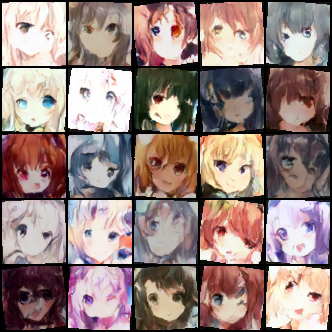
...Boss baseline(FID ≤ 9000, AFD ≥ 0.6)
- StyleGAN
仅供参考,从实验结果上来看,扩散模型生成的图像视觉上更清晰,而 StyleGAN 的风格更一致。
当然,同样存在设置出现问题的情况(毕竟超参数直接延续了之前的设定。Anyway,希望对你有所帮助)
| Strong (DDPM) | Boss (StyleGAN) |
|---|---|
 |  |
class StyleGANTrainer(object):def __init__(self, folder, image_size, *,train_batch_size=16, gradient_accumulate_every=1, train_lr=1e-3, train_num_steps=100000, ema_update_every=10, ema_decay=0.995, save_and_sample_every=1000, num_samples=25, results_folder='./results', split_batches=True):super().__init__()dataloader_config = DataLoaderConfiguration(split_batches=split_batches)self.accelerator = Accelerator(dataloader_config=dataloader_config,mixed_precision='no')self.image_size = image_size# Initialize the generator and discriminatorself.gen = self.create_generator().cuda()self.dis = self.create_discriminator().cuda()self.g_optim = torch.optim.Adam(self.gen.parameters(), lr=train_lr, betas=(0.0, 0.99))self.d_optim = torch.optim.Adam(self.dis.parameters(), lr=train_lr, betas=(0.0, 0.99))self.train_num_steps = train_num_stepsself.batch_size = train_batch_sizeself.gradient_accumulate_every = gradient_accumulate_every# Initialize the dataset and dataloaderself.ds = Dataset(folder, image_size)self.dl = cycle(DataLoader(self.ds, batch_size=train_batch_size, shuffle=True, pin_memory=True, num_workers=os.cpu_count()))# Initialize the EMA for the generatorself.ema = EMA(self.gen, beta=ema_decay, update_every=ema_update_every).to(self.device)self.results_folder = Path(results_folder)self.results_folder.mkdir(exist_ok=True)self.save_and_sample_every = save_and_sample_everyself.num_samples = num_samplesself.step = 0def create_generator(self):return dnnlib.util.construct_class_by_name(class_name='training.networks.Generator',z_dim=512,c_dim=0,w_dim=512,img_resolution=self.image_size,img_channels=3)def create_discriminator(self):return dnnlib.util.construct_class_by_name(class_name='training.networks.Discriminator',c_dim=0,img_resolution=self.image_size,img_channels=3)@propertydef device(self):return self.accelerator.devicedef save(self, milestone):if not self.accelerator.is_local_main_process:returndata = {'step': self.step,'gen': self.accelerator.get_state_dict(self.gen),'dis': self.accelerator.get_state_dict(self.dis),'g_optim': self.g_optim.state_dict(),'d_optim': self.d_optim.state_dict(),'ema': self.ema.state_dict()}torch.save(data, str(self.results_folder / f'model-{milestone}.pt'))def load(self, ckpt):data = torch.load(ckpt, map_location=self.device)self.gen.load_state_dict(data['gen'])self.dis.load_state_dict(data['dis'])self.g_optim.load_state_dict(data['g_optim'])self.d_optim.load_state_dict(data['d_optim'])self.ema.load_state_dict(data['ema'])self.step = data['step']def train(self):with tqdm(initial=self.step, total=self.train_num_steps, disable=not self.accelerator.is_main_process) as pbar:while self.step < self.train_num_steps:total_g_loss = 0.total_d_loss = 0.for _ in range(self.gradient_accumulate_every):# Get a batch of real imagesreal_images = next(self.dl).to(self.device)# Generate latent vectorslatent = torch.randn([self.batch_size, self.gen.z_dim]).cuda()# Generate fake imagesfake_images = self.gen(latent, None)# Discriminator logits for real and fake imagesreal_logits = self.dis(real_images, None)fake_logits = self.dis(fake_images.detach(), None)# Discriminator lossd_loss = torch.nn.functional.softplus(fake_logits).mean() + torch.nn.functional.softplus(-real_logits).mean()# Update discriminatorself.d_optim.zero_grad()self.accelerator.backward(d_loss / self.gradient_accumulate_every)self.d_optim.step()total_d_loss += d_loss.item()# Generator logits for fake imagesfake_logits = self.dis(fake_images, None)# Generator lossg_loss = torch.nn.functional.softplus(-fake_logits).mean()# Update generatorself.g_optim.zero_grad()self.accelerator.backward(g_loss / self.gradient_accumulate_every)self.g_optim.step()total_g_loss += g_loss.item()self.ema.update()pbar.set_description(f'G loss: {total_g_loss:.4f} D loss: {total_d_loss:.4f}')self.step += 1if self.step % self.save_and_sample_every == 0:self.ema.ema_model.eval()with torch.no_grad():milestone = self.step // self.save_and_sample_everybatches = num_to_groups(self.num_samples, self.batch_size)all_images_list = list(map(lambda n: self.ema.ema_model(torch.randn([n, self.gen.z_dim]).cuda(), None), batches))all_images = torch.cat(all_images_list, dim=0)utils.save_image(all_images, str(self.results_folder / f'sample-{milestone}.png'), nrow=int(np.sqrt(self.num_samples)))self.save(milestone)pbar.update(1)print('Training complete')def inference(self, num=1000, n_iter=5, output_path='./submission'):if not os.path.exists(output_path):os.mkdir(output_path)with torch.no_grad():for i in range(n_iter):latent = torch.randn(num // n_iter, self.gen.z_dim).cuda()images = self.ema.ema_model(latent, None)for j, img in enumerate(images):utils.save_image(img, f'{output_path}/{i * (num // n_iter) + j + 1}.jpg')完整的样例图对比
| Simple | Medium | Strong | Boss |
|---|---|---|---|
 |  |  | 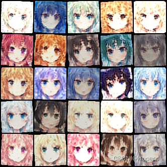 |