文章目录
- CIFAR10数据集介绍
- 1. 数据的下载
- 2.修改模型与前面的参数设置保持一致
- 3. 新建模型
- 4. 从数据集中分批量读取数据
- 5. 定义损失函数
- 6. 定义优化器
- 7. 开始训练
- 8.测试模型
- 9. 手写体图片的可视化
- 10. 多幅图片的可视化
- 思考题
- 11. 读取测试集的图片预测值(神经网络的输出为10)
- 12. 采用pandas可视化数据
- 13. 对预测错误的样本点进行可视化
- 14. 看看错误样本被预测为哪些数据?
- 15.输出错误的模型类别
CIFAR10数据集介绍
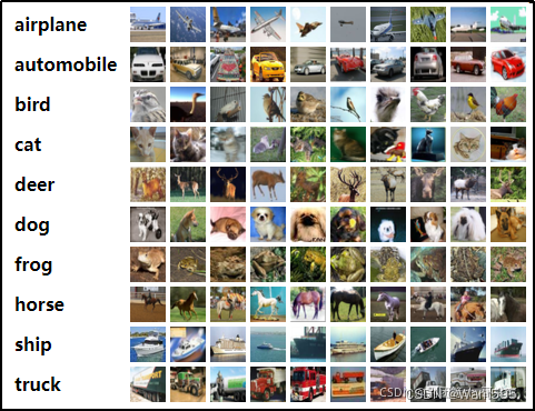
CIFAR-10 数据集由10个类别的60000张32x32彩色图像组成,每类6000张图像。有50000张训练图像和10000张测试图像。数据集分为五个训练批次
和一个测试批次,每个批次有10000张图像。测试批次包含从每个类别中随机选择的1000张图像。训练批次包含随机顺序的剩余图像,但一些训练批次
可能包含比另一个类别更多的图像。在它们之间训练批次包含来自每个类的5000张图像。以下是数据集中的类,以及每个类中的10张随机图像:
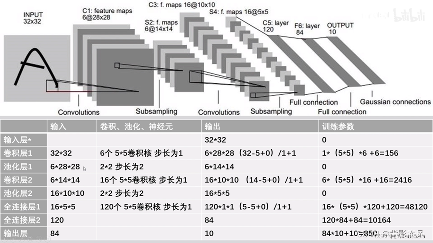
因为CIFAR10数据集颜色通道有3个,所以卷积层L1的输入通道数量(in_channels)需要设为3。全连接层fc1的输入维度设为400,这与上例设为256有所不同,原因是初始输入数据的形状不一样,经过卷积池化后,输出的数据形状是不一样的。如果是采用动态图开发模型,那么有一种便捷的方式查看中间结果的形状,即在forward()方法中,用print函数把中间结果的形状打印出来。根据中间结果的形状,决定接下来各网络层的参数。
1. 数据的下载
import torch
import torchvision.transforms as transforms
from torchvision.datasets import CIFAR10
train_dataset = CIFAR10(root="./data/CIFAR10",train=True,transform=transforms.ToTensor(),download=True)
test_dataset = CIFAR10(root="./data/CIFAR10", train=False,transform=transforms.ToTensor())
Files already downloaded and verified
train_dataset[0][0].shape
torch.Size([3, 32, 32])
train_dataset[0][1]
6
2.修改模型与前面的参数设置保持一致
from torch import nn
class Lenet5(nn.Module):def __init__(self):super(Lenet5,self).__init__()#1+ 32-5/(1)==28self.features=nn.Sequential(#定义第一个卷积层nn.Conv2d(in_channels=3,out_channels=6,kernel_size=(5,5),stride=1),nn.ReLU(),nn.AvgPool2d(kernel_size=2,stride=2),#定义第二个卷积层nn.Conv2d(in_channels=6,out_channels=16,kernel_size=(5,5),stride=1),nn.ReLU(),nn.MaxPool2d(kernel_size=2,stride=2),)#定义全连接层self.classfier=nn.Sequential(nn.Linear(in_features=400,out_features=120),nn.ReLU(),nn.Linear(in_features=120,out_features=84),nn.ReLU(),nn.Linear(in_features=84,out_features=10), )def forward(self,x):x=self.features(x)x=torch.flatten(x,1)result=self.classfier(x)return result
3. 新建模型
model=Lenet5()
device=torch.device("cuda:0" if torch.cuda.is_available() else "cpu")
model=model.to(device)
4. 从数据集中分批量读取数据
#加载数据集
batch_size=32
train_loader= torch.utils.data.DataLoader(train_dataset, batch_size, shuffle=True)
test_loader= torch.utils.data.DataLoader(test_dataset, batch_size, shuffle=False)
# 类别信息也是需要我们给定的
classes = ('plane', 'car', 'bird', 'cat','deer', 'dog', 'frog', 'horse', 'ship', 'truck')
5. 定义损失函数
from torch import optim
loss_fun=nn.CrossEntropyLoss()
loss_lst=[]
6. 定义优化器
optimizer=optim.SGD(params=model.parameters(),lr=0.001,momentum=0.9)
7. 开始训练
import time
start_time=time.time()
#训练的迭代次数
for epoch in range(10):loss_i=0for i,(batch_data,batch_label) in enumerate(train_loader):#清空优化器的梯度optimizer.zero_grad()#模型前向预测pred=model(batch_data)loss=loss_fun(pred,batch_label)loss_i+=lossloss.backward()optimizer.step()if (i+1)%200==0:print("第%d次训练,第%d批次,损失为%.2f"%(epoch,i,loss_i/200))loss_i=0
end_time=time.time()
print("共训练了%d 秒"%(end_time-start_time))
第0次训练,第199批次,损失为2.30
第0次训练,第399批次,损失为2.30
第0次训练,第599批次,损失为2.30
第0次训练,第799批次,损失为2.30
第0次训练,第999批次,损失为2.30
第0次训练,第1199批次,损失为2.30
第0次训练,第1399批次,损失为2.30
第1次训练,第199批次,损失为2.30
第1次训练,第399批次,损失为2.30
第1次训练,第599批次,损失为2.30
第1次训练,第799批次,损失为2.30
第1次训练,第999批次,损失为2.29
第1次训练,第1199批次,损失为2.27
第1次训练,第1399批次,损失为2.18
第2次训练,第199批次,损失为2.07
第2次训练,第399批次,损失为2.04
第2次训练,第599批次,损失为2.03
第2次训练,第799批次,损失为2.00
第2次训练,第999批次,损失为1.98
第2次训练,第1199批次,损失为1.96
第2次训练,第1399批次,损失为1.95
第3次训练,第199批次,损失为1.89
第3次训练,第399批次,损失为1.86
第3次训练,第599批次,损失为1.84
第3次训练,第799批次,损失为1.80
第3次训练,第999批次,损失为1.75
第3次训练,第1199批次,损失为1.71
第3次训练,第1399批次,损失为1.71
第4次训练,第199批次,损失为1.66
第4次训练,第399批次,损失为1.65
第4次训练,第599批次,损失为1.63
第4次训练,第799批次,损失为1.61
第4次训练,第999批次,损失为1.62
第4次训练,第1199批次,损失为1.60
第4次训练,第1399批次,损失为1.59
第5次训练,第199批次,损失为1.56
第5次训练,第399批次,损失为1.56
第5次训练,第599批次,损失为1.54
第5次训练,第799批次,损失为1.55
第5次训练,第999批次,损失为1.52
第5次训练,第1199批次,损失为1.52
第5次训练,第1399批次,损失为1.49
第6次训练,第199批次,损失为1.50
第6次训练,第399批次,损失为1.47
第6次训练,第599批次,损失为1.46
第6次训练,第799批次,损失为1.47
第6次训练,第999批次,损失为1.46
第6次训练,第1199批次,损失为1.43
第6次训练,第1399批次,损失为1.45
第7次训练,第199批次,损失为1.42
第7次训练,第399批次,损失为1.42
第7次训练,第599批次,损失为1.39
第7次训练,第799批次,损失为1.39
第7次训练,第999批次,损失为1.40
第7次训练,第1199批次,损失为1.40
第7次训练,第1399批次,损失为1.40
第8次训练,第199批次,损失为1.36
第8次训练,第399批次,损失为1.37
第8次训练,第599批次,损失为1.38
第8次训练,第799批次,损失为1.37
第8次训练,第999批次,损失为1.34
第8次训练,第1199批次,损失为1.37
第8次训练,第1399批次,损失为1.35
第9次训练,第199批次,损失为1.31
第9次训练,第399批次,损失为1.31
第9次训练,第599批次,损失为1.31
第9次训练,第799批次,损失为1.31
第9次训练,第999批次,损失为1.34
第9次训练,第1199批次,损失为1.32
第9次训练,第1399批次,损失为1.31
共训练了156 秒
8.测试模型
len(test_dataset)
10000
correct=0
for batch_data,batch_label in test_loader:pred_test=model(batch_data)pred_result=torch.max(pred_test.data,1)[1]correct+=(pred_result==batch_label).sum()
print("准确率为:%.2f%%"%(correct/len(test_dataset)))
准确率为:0.53%
9. 手写体图片的可视化
from torchvision import transforms as T
import torch
len(train_dataset)
50000
train_dataset[0][0].shape
torch.Size([3, 32, 32])
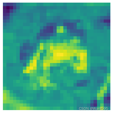
import matplotlib.pyplot as plt
plt.imshow(train_dataset[0][0][0],cmap="gray")
plt.axis('off')
(-0.5, 31.5, 31.5, -0.5)
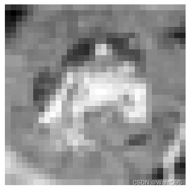
plt.imshow(train_dataset[0][0][0])
plt.axis('off')
(-0.5, 31.5, 31.5, -0.5)
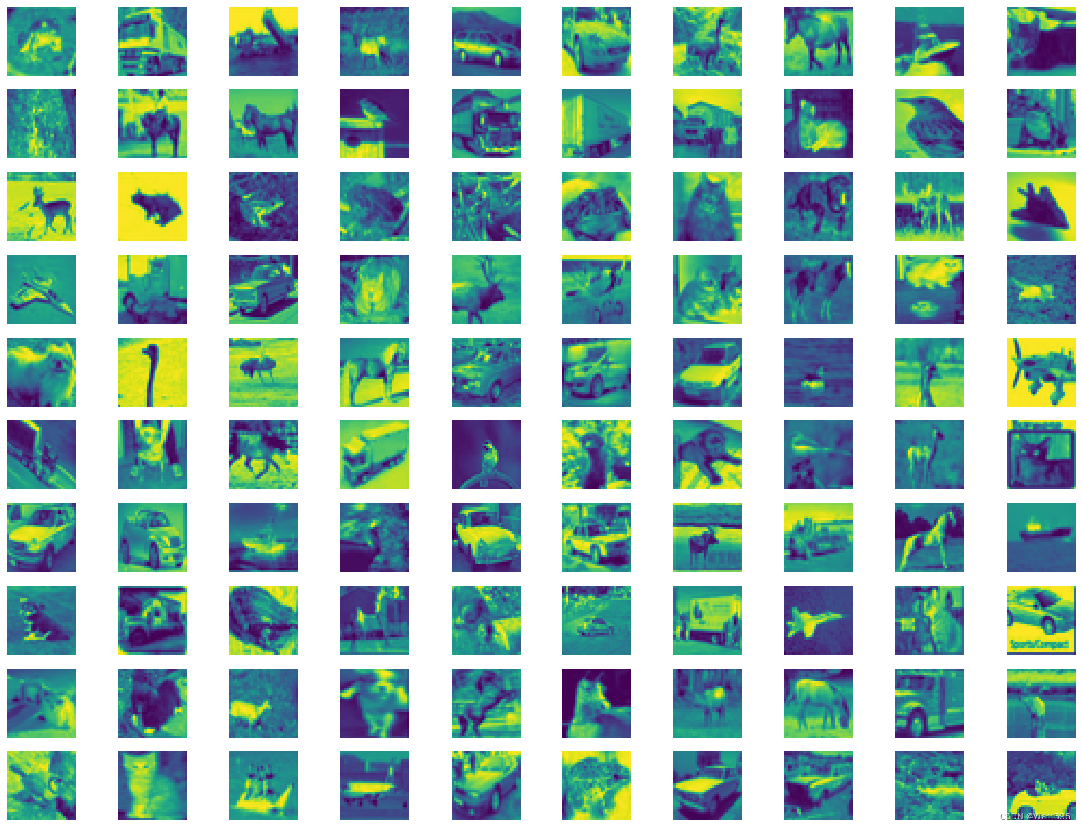
10. 多幅图片的可视化
from matplotlib import pyplot as plt
plt.figure(figsize=(20,15))
cols=10
rows=10
for i in range(0,rows):for j in range(0,cols):idx=j+i*colsplt.subplot(rows,cols,idx+1) plt.imshow(train_dataset[idx][0][0])plt.axis('off')
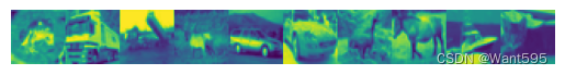
import numpy as np
img10 = np.stack(list(train_dataset[i][0][0] for i in range(10)), axis=1).reshape(32,320)
plt.imshow(img10)
plt.axis('off')
(-0.5, 319.5, 31.5, -0.5)
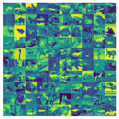
img100 = np.stack( tuple( np.stack(tuple( train_dataset[j*10+i][0][0] for i in range(10) ), axis=1).reshape(32,320) for j in range(10)),axis=0).reshape(320,320)
plt.imshow(img100)
plt.axis('off')
(-0.5, 319.5, 319.5, -0.5)
思考题
- 测试集中有哪些识别错误的手写数字图片? 汇集整理并分析原因?
11. 读取测试集的图片预测值(神经网络的输出为10)
pre_result=torch.zeros(len(test_dataset),10)
for i in range(len(test_dataset)):pre_result[i,:]=model(torch.reshape(test_dataset[i][0],(-1,3,32,32)))
pre_result
tensor([[-0.4934, -1.0982, 0.4072, ..., -0.4038, -1.1655, -0.8201],[ 4.0154, 4.4736, -0.2921, ..., -2.3925, 4.3176, 4.1910],[ 1.3858, 3.2022, -0.7004, ..., -2.2767, 3.0923, 2.3740],...,[-1.9551, -3.8085, 1.7917, ..., 2.1104, -2.9573, -1.7387],[ 0.6681, -0.5328, 0.3059, ..., 0.1170, -2.5236, -0.5746],[-0.5194, -2.6185, 1.1929, ..., 3.7749, -2.3134, -1.5123]],grad_fn=<CopySlices>)
pre_result.shape
torch.Size([10000, 10])
pre_result[:5]
tensor([[-0.4934, -1.0982, 0.4072, 1.7331, -0.4456, 1.6433, 0.1721, -0.4038,-1.1655, -0.8201],[ 4.0154, 4.4736, -0.2921, -3.2882, -1.6234, -4.4814, -3.1241, -2.3925,4.3176, 4.1910],[ 1.3858, 3.2022, -0.7004, -1.0123, -1.7394, -1.6657, -3.2578, -2.2767,3.0923, 2.3740],[ 2.1151, 0.8262, 0.0071, -1.1410, -0.3051, -2.0239, -2.3023, -0.3573,2.9400, 0.5595],[-2.3524, -2.7907, 1.9834, 2.1088, 2.7645, 1.1118, 2.9782, -0.3876,-3.2325, -2.3916]], grad_fn=<SliceBackward0>)
#显示这10000张图片的标签
label_10000=[test_dataset[i][1] for i in range(10000)]
label_10000
[3,8,8,0,6,6,1,6,3,1,0,9,5,7,9,8,5,7,8,6,7,0,4,9,5,2,4,0,9,6,6,5,4,5,9,2,4,1,9,5,4,6,5,6,0,9,3,9,7,6,9,8,0,3,8,8,7,7,4,6,7,3,6,3,6,2,1,2,3,7,2,6,8,8,0,2,9,3,3,8,8,1,1,7,2,5,2,7,8,9,0,3,8,6,4,6,6,0,0,7,4,5,6,3,1,1,3,6,8,7,4,0,6,2,1,3,0,4,2,7,8,3,1,2,8,0,8,3,5,2,4,1,8,9,1,2,9,7,2,9,6,5,6,3,8,7,6,2,5,2,8,9,6,0,0,5,2,9,5,4,2,1,6,6,8,4,8,4,5,0,9,9,9,8,9,9,3,7,5,0,0,5,2,2,3,8,6,3,4,0,5,8,0,1,7,2,8,8,7,8,5,1,8,7,1,3,0,5,7,9,7,4,5,9,8,0,7,9,8,2,7,6,9,4,3,9,6,4,7,6,5,1,5,8,8,0,4,0,5,5,1,1,8,9,0,3,1,9,2,2,5,3,9,9,4,0,3,0,0,9,8,1,5,7,0,8,2,4,7,0,2,3,6,3,8,5,0,3,4,3,9,0,6,1,0,9,1,0,7,9,1,2,6,9,3,4,6,0,0,6,6,6,3,2,6,1,8,2,1,6,8,6,8,0,4,0,7,7,5,5,3,5,2,3,4,1,7,5,4,6,1,9,3,6,6,9,3,8,0,7,2,6,2,5,8,5,4,6,8,9,9,1,0,2,2,7,3,2,8,0,9,5,8,1,9,4,1,3,8,1,4,7,9,4,2,7,0,7,0,6,6,9,0,9,2,8,7,2,2,5,1,2,6,2,9,6,2,3,0,3,9,8,7,8,8,4,0,1,8,2,7,9,3,6,1,9,0,7,3,7,4,5,0,0,2,9,3,4,0,6,2,5,3,7,3,7,2,5,3,1,1,4,9,9,5,7,5,0,2,2,2,9,7,3,9,4,3,5,4,6,5,6,1,4,3,4,4,3,7,8,3,7,8,0,5,7,6,0,5,4,8,6,8,5,5,9,9,9,5,0,1,0,8,1,1,8,0,2,2,0,4,6,5,4,9,4,7,9,9,4,5,6,6,1,5,3,8,9,5,8,5,7,0,7,0,5,0,0,4,6,9,0,9,5,6,6,6,2,9,0,1,7,6,7,5,9,1,6,2,5,5,5,8,5,9,4,6,4,3,2,0,7,6,2,2,3,9,7,9,2,6,7,1,3,6,6,8,9,7,5,4,0,8,4,0,9,3,4,8,9,6,9,2,6,1,4,7,3,5,3,8,5,0,2,1,6,4,3,3,9,6,9,8,8,5,8,6,6,2,1,7,7,1,2,7,9,9,4,4,1,2,5,6,8,7,6,8,3,0,5,5,3,0,7,9,1,3,4,4,5,3,9,5,6,9,2,1,1,4,1,9,4,7,6,3,8,9,0,1,3,6,3,6,3,2,0,3,1,0,5,9,6,4,8,9,6,9,6,3,0,3,2,2,7,8,3,8,2,7,5,7,2,4,8,7,4,2,9,8,8,6,8,8,7,4,3,3,8,4,9,4,8,8,1,8,2,1,3,6,5,4,2,7,9,9,4,1,4,1,3,2,7,0,7,9,7,6,6,2,5,9,2,9,1,2,2,6,8,2,1,3,6,6,0,1,2,7,0,5,4,6,1,6,4,0,2,2,6,0,5,9,1,7,6,7,0,3,9,6,8,3,0,3,4,7,7,1,4,7,2,7,1,4,7,4,4,8,4,7,7,5,3,7,2,0,8,9,5,8,3,6,2,0,8,7,3,7,6,5,3,1,3,2,2,5,4,1,2,9,2,7,0,7,2,1,3,2,0,2,4,7,9,8,9,0,7,7,0,7,8,4,6,3,3,0,1,3,7,0,1,3,1,4,2,3,8,4,2,3,7,8,4,3,0,9,0,0,1,0,4,4,6,7,6,1,1,3,7,3,5,2,6,6,5,8,7,1,6,8,8,5,3,0,4,0,1,3,8,8,0,6,9,9,9,5,5,8,6,0,0,4,2,3,2,7,2,2,5,9,8,9,1,7,4,0,3,0,1,3,8,3,9,6,1,4,7,0,3,7,8,9,1,1,6,6,6,6,9,1,9,9,4,2,1,7,0,6,8,1,9,2,9,0,4,7,8,3,1,2,0,1,5,8,4,6,3,8,1,3,8,...]
import numpy
pre_10000=pre_result.detach()
pre_10000
tensor([[-0.4934, -1.0982, 0.4072, ..., -0.4038, -1.1655, -0.8201],[ 4.0154, 4.4736, -0.2921, ..., -2.3925, 4.3176, 4.1910],[ 1.3858, 3.2022, -0.7004, ..., -2.2767, 3.0923, 2.3740],...,[-1.9551, -3.8085, 1.7917, ..., 2.1104, -2.9573, -1.7387],[ 0.6681, -0.5328, 0.3059, ..., 0.1170, -2.5236, -0.5746],[-0.5194, -2.6185, 1.1929, ..., 3.7749, -2.3134, -1.5123]])
pre_10000=numpy.array(pre_10000)
pre_10000
array([[-0.49338394, -1.098238 , 0.40724754, ..., -0.40375623,-1.165497 , -0.820113 ],[ 4.0153656 , 4.4736323 , -0.29209492, ..., -2.392501 ,4.317573 , 4.190993 ],[ 1.3858219 , 3.2021556 , -0.70040375, ..., -2.2767155 ,3.092283 , 2.373978 ],...,[-1.9550545 , -3.808494 , 1.7917161 , ..., 2.110389 ,-2.9572597 , -1.7386926 ],[ 0.66809845, -0.5327946 , 0.30590305, ..., 0.11701592,-2.5236375 , -0.5746133 ],[-0.51935434, -2.6184506 , 1.1929085 , ..., 3.7748828 ,-2.3134274 , -1.5123445 ]], dtype=float32)
12. 采用pandas可视化数据
import pandas as pd
table=pd.DataFrame(zip(pre_10000,label_10000))
table
| 0 | 1 | |
|---|---|---|
| 0 | [-0.49338394, -1.098238, 0.40724754, 1.7330961... | 3 |
| 1 | [4.0153656, 4.4736323, -0.29209492, -3.2882178... | 8 |
| 2 | [1.3858219, 3.2021556, -0.70040375, -1.0123051... | 8 |
| 3 | [2.11508, 0.82618773, 0.007076204, -1.1409527,... | 0 |
| 4 | [-2.352432, -2.7906854, 1.9833877, 2.1087575, ... | 6 |
| ... | ... | ... |
| 9995 | [-0.55809855, -4.3891077, -0.3040389, 3.001731... | 8 |
| 9996 | [-2.7151718, -4.1596007, 1.2393914, 2.8491826,... | 3 |
| 9997 | [-1.9550545, -3.808494, 1.7917161, 2.6365147, ... | 5 |
| 9998 | [0.66809845, -0.5327946, 0.30590305, -0.182045... | 1 |
| 9999 | [-0.51935434, -2.6184506, 1.1929085, 0.1288419... | 7 |
10000 rows × 2 columns
table[0].values
array([array([-0.49338394, -1.098238 , 0.40724754, 1.7330961 , -0.4455951 ,1.6433077 , 0.1720748 , -0.40375623, -1.165497 , -0.820113 ],dtype=float32) ,array([ 4.0153656 , 4.4736323 , -0.29209492, -3.2882178 , -1.6234205 ,-4.481386 , -3.1240807 , -2.392501 , 4.317573 , 4.190993 ],dtype=float32) ,array([ 1.3858219 , 3.2021556 , -0.70040375, -1.0123051 , -1.7393746 ,-1.6656632 , -3.2578242 , -2.2767155 , 3.092283 , 2.373978 ],dtype=float32) ,...,array([-1.9550545 , -3.808494 , 1.7917161 , 2.6365147 , 0.37311587,3.545672 , -0.43889195, 2.110389 , -2.9572597 , -1.7386926 ],dtype=float32) ,array([ 0.66809845, -0.5327946 , 0.30590305, -0.18204585, 2.0045712 ,0.47369143, -0.3122899 , 0.11701592, -2.5236375 , -0.5746133 ],dtype=float32) ,array([-0.51935434, -2.6184506 , 1.1929085 , 0.1288419 , 1.8770852 ,0.4296908 , -0.22015049, 3.7748828 , -2.3134274 , -1.5123445 ],dtype=float32) ],dtype=object)
table["pred"]=[np.argmax(table[0][i]) for i in range(table.shape[0])]
table
| 0 | 1 | pred | |
|---|---|---|---|
| 0 | [-0.49338394, -1.098238, 0.40724754, 1.7330961... | 3 | 3 |
| 1 | [4.0153656, 4.4736323, -0.29209492, -3.2882178... | 8 | 1 |
| 2 | [1.3858219, 3.2021556, -0.70040375, -1.0123051... | 8 | 1 |
| 3 | [2.11508, 0.82618773, 0.007076204, -1.1409527,... | 0 | 8 |
| 4 | [-2.352432, -2.7906854, 1.9833877, 2.1087575, ... | 6 | 6 |
| ... | ... | ... | ... |
| 9995 | [-0.55809855, -4.3891077, -0.3040389, 3.001731... | 8 | 5 |
| 9996 | [-2.7151718, -4.1596007, 1.2393914, 2.8491826,... | 3 | 3 |
| 9997 | [-1.9550545, -3.808494, 1.7917161, 2.6365147, ... | 5 | 5 |
| 9998 | [0.66809845, -0.5327946, 0.30590305, -0.182045... | 1 | 4 |
| 9999 | [-0.51935434, -2.6184506, 1.1929085, 0.1288419... | 7 | 7 |
10000 rows × 3 columns
13. 对预测错误的样本点进行可视化
mismatch=table[table[1]!=table["pred"]]
mismatch
| 0 | 1 | pred | |
|---|---|---|---|
| 1 | [4.0153656, 4.4736323, -0.29209492, -3.2882178... | 8 | 1 |
| 2 | [1.3858219, 3.2021556, -0.70040375, -1.0123051... | 8 | 1 |
| 3 | [2.11508, 0.82618773, 0.007076204, -1.1409527,... | 0 | 8 |
| 8 | [0.02641207, -3.6653092, 2.294829, 2.2884543, ... | 3 | 5 |
| 12 | [-1.4556388, -1.7955011, -0.6100754, 1.169481,... | 5 | 6 |
| ... | ... | ... | ... |
| 9989 | [-0.2553262, -2.8777533, 3.4579017, 0.3079242,... | 2 | 4 |
| 9993 | [-0.077826336, -3.14616, 0.8994149, 3.5604722,... | 5 | 3 |
| 9994 | [-1.2543154, -2.4472265, 0.6754027, 2.0582433,... | 3 | 6 |
| 9995 | [-0.55809855, -4.3891077, -0.3040389, 3.001731... | 8 | 5 |
| 9998 | [0.66809845, -0.5327946, 0.30590305, -0.182045... | 1 | 4 |
4657 rows × 3 columns
from matplotlib import pyplot as plt
plt.scatter(mismatch[1],mismatch["pred"])
<matplotlib.collections.PathCollection at 0x1b3a92ef910>
14. 看看错误样本被预测为哪些数据?
mismatch[mismatch[1]==9].sort_values("pred").index
Int64Index([2129, 1465, 2907, 787, 2902, 2307, 4588, 5737, 8276, 8225,...7635, 7553, 7526, 3999, 1626, 1639, 4193, 7198, 3957, 3344],dtype='int64', length=396)
idx_lst=mismatch[mismatch[1]==9].sort_values("pred").index.values
idx_lst,len(idx_lst)
(array([2129, 1465, 2907, 787, 2902, 2307, 4588, 5737, 8276, 8225, 8148,4836, 1155, 7218, 8034, 7412, 5069, 1629, 5094, 5109, 7685, 5397,1427, 5308, 8727, 2960, 2491, 6795, 1997, 6686, 9449, 6545, 8985,9401, 3564, 6034, 383, 9583, 9673, 507, 3288, 6868, 9133, 9085,577, 4261, 6974, 411, 6290, 5416, 5350, 5950, 5455, 5498, 6143,5964, 5864, 5877, 6188, 5939, 14, 5300, 3501, 3676, 3770, 3800,3850, 3893, 3902, 4233, 4252, 4253, 4276, 5335, 4297, 4418, 4445,4536, 4681, 6381, 4929, 4945, 5067, 5087, 5166, 5192, 4364, 4928,7024, 6542, 8144, 8312, 8385, 8406, 8453, 8465, 8521, 8585, 8673,8763, 8946, 9067, 9069, 9199, 9209, 9217, 9280, 9403, 9463, 9518,9692, 9743, 9871, 9875, 9881, 8066, 6509, 8057, 7826, 6741, 6811,6814, 6840, 6983, 7007, 3492, 7028, 7075, 7121, 7232, 7270, 7424,7431, 7444, 7492, 7499, 7501, 7578, 7639, 7729, 7767, 7792, 7818,7824, 7942, 3459, 4872, 1834, 1487, 1668, 1727, 1732, 1734, 1808,1814, 1815, 1831, 1927, 2111, 2126, 2190, 2246, 2290, 2433, 2596,2700, 2714, 1439, 1424, 1376, 1359, 28, 151, 172, 253, 259,335, 350, 591, 625, 2754, 734, 940, 951, 970, 1066, 1136,1177, 1199, 1222, 1231, 853, 2789, 9958, 2946, 3314, 3307, 2876,3208, 3166, 2944, 2817, 2305, 7522, 7155, 7220, 4590, 2899, 2446,2186, 7799, 9492, 3163, 4449, 2027, 2387, 1064, 3557, 2177, 654,9791, 2670, 2514, 2495, 3450, 8972, 3210, 3755, 2756, 7967, 3970,4550, 6017, 938, 744, 6951, 3397, 4852, 3133, 7931, 707, 3312,7470, 6871, 8292, 7100, 9529, 9100, 3853, 9060, 9732, 2521, 3789,2974, 5311, 3218, 5736, 3055, 7076, 1220, 9147, 1344, 532, 8218,3569, 1008, 8475, 8877, 1582, 8936, 4758, 1837, 9517, 252, 5832,1916, 6369, 4979, 9324, 6218, 9777, 7923, 4521, 2868, 213, 8083,5952, 5579, 4508, 5488, 2460, 5332, 5180, 8323, 8345, 3776, 2568,5151, 4570, 2854, 8488, 4874, 680, 2810, 1285, 6136, 3339, 9143,6852, 1906, 7067, 7073, 2975, 1924, 6804, 6755, 9299, 2019, 9445,9560, 360, 1601, 7297, 9122, 6377, 9214, 6167, 3980, 394, 7491,7581, 9349, 8953, 222, 139, 530, 3577, 9868, 247, 9099, 9026,209, 538, 3229, 9258, 585, 9204, 9643, 1492, 3609, 6570, 6561,6469, 6435, 6419, 2155, 6275, 4481, 2202, 1987, 2271, 2355, 2366,2432, 5400, 2497, 2727, 4931, 4619, 9884, 5902, 8796, 6848, 6960,8575, 8413, 981, 8272, 8145, 3172, 1221, 3168, 1256, 1889, 1291,3964, 7635, 7553, 7526, 3999, 1626, 1639, 4193, 7198, 3957, 3344],dtype=int64),396)
import numpy as np
img=np.stack(list(test_dataset[idx_lst[i]][0][0] for i in range(5)),axis=1).reshape(32,32*5)
plt.imshow(img)
plt.axis('off')
(-0.5, 159.5, 31.5, -0.5)
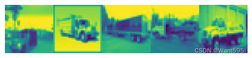
#显示4行
import numpy as np
img20=np.stack(tuple(np.stack(tuple(test_dataset[idx_lst[i+j*5]][0][0] for i in range(5)),axis=1).reshape(32,32*5) for j in range(4)),axis=0).reshape(32*4,32*5)
plt.imshow(img20)
plt.axis('off')
(-0.5, 159.5, 127.5, -0.5)

15.输出错误的模型类别
idx_lst=mismatch[mismatch[1]==9].index.values
table.iloc[idx_lst[:], 2].values
array([1, 1, 8, 1, 1, 8, 7, 8, 8, 6, 1, 1, 1, 1, 7, 0, 7, 0, 0, 8, 6, 8,0, 8, 1, 1, 3, 7, 5, 1, 4, 0, 1, 4, 1, 1, 1, 8, 6, 3, 1, 1, 0, 1,1, 6, 8, 1, 1, 8, 7, 8, 6, 1, 1, 1, 0, 1, 0, 1, 8, 6, 7, 8, 0, 8,1, 1, 1, 1, 1, 1, 1, 1, 1, 6, 8, 7, 6, 7, 1, 8, 0, 7, 3, 1, 1, 0,8, 3, 3, 1, 8, 1, 8, 1, 2, 0, 8, 8, 3, 8, 1, 3, 7, 0, 3, 8, 3, 5,7, 1, 3, 1, 1, 8, 1, 3, 1, 7, 1, 7, 7, 1, 3, 0, 0, 1, 1, 0, 5, 7,6, 4, 3, 1, 8, 8, 1, 3, 5, 8, 0, 1, 5, 1, 7, 8, 4, 3, 1, 1, 1, 3,0, 6, 8, 8, 1, 3, 1, 7, 5, 1, 1, 5, 1, 1, 8, 8, 4, 7, 8, 8, 1, 1,1, 0, 1, 1, 1, 1, 1, 3, 8, 7, 7, 1, 4, 7, 0, 2, 8, 1, 6, 0, 4, 1,7, 1, 1, 8, 1, 6, 1, 0, 1, 0, 0, 7, 1, 7, 1, 1, 0, 5, 7, 1, 1, 0,8, 1, 1, 7, 1, 7, 5, 0, 6, 1, 1, 8, 1, 1, 7, 1, 4, 0, 7, 1, 7, 1,6, 8, 1, 6, 7, 1, 8, 8, 8, 1, 1, 0, 8, 8, 0, 1, 7, 0, 7, 1, 1, 1,8, 7, 0, 5, 4, 8, 0, 1, 1, 1, 1, 7, 7, 1, 6, 5, 1, 2, 8, 0, 2, 1,1, 7, 0, 1, 1, 1, 5, 7, 1, 1, 1, 2, 8, 8, 1, 7, 8, 1, 0, 1, 1, 1,3, 1, 1, 1, 7, 4, 1, 4, 0, 1, 1, 7, 1, 8, 0, 6, 0, 8, 0, 5, 1, 7,7, 1, 1, 8, 1, 1, 6, 7, 1, 8, 1, 1, 0, 1, 8, 6, 6, 1, 8, 3, 0, 8,5, 1, 1, 0, 8, 5, 7, 0, 7, 6, 1, 8, 1, 7, 1, 8, 1, 7, 6, 8, 0, 1,7, 0, 1, 3, 6, 1, 5, 7, 0, 8, 0, 1, 5, 1, 6, 3, 8, 1, 1, 1, 8, 1],dtype=int64)
arr2=table.iloc[idx_lst[:], 2].values
print('错误模型共' + str(len(arr2)) + '个')
for i in range(33):for j in range(12):print(classes[arr2[j+i*12]],end=" ")print()
错误模型共396个
car car ship car car ship horse ship ship frog car car
car car horse plane horse plane plane ship frog ship plane ship
car car cat horse dog car deer plane car deer car car
car ship frog cat car car plane car car frog ship car
car ship horse ship frog car car car plane car plane car
ship frog horse ship plane ship car car car car car car
car car car frog ship horse frog horse car ship plane horse
cat car car plane ship cat cat car ship car ship car
bird plane ship ship cat ship car cat horse plane cat ship
cat dog horse car cat car car ship car cat car horse
car horse horse car cat plane plane car car plane dog horse
frog deer cat car ship ship car cat dog ship plane car
dog car horse ship deer cat car car car cat plane frog
ship ship car cat car horse dog car car dog car car
ship ship deer horse ship ship car car car plane car car
car car car cat ship horse horse car deer horse plane bird
ship car frog plane deer car horse car car ship car frog
car plane car plane plane horse car horse car car plane dog
horse car car plane ship car car horse car horse dog plane
frog car car ship car car horse car deer plane horse car
horse car frog ship car frog horse car ship ship ship car
car plane ship ship plane car horse plane horse car car car
ship horse plane dog deer ship plane car car car car horse
horse car frog dog car bird ship plane bird car car horse
plane car car car dog horse car car car bird ship ship
car horse ship car plane car car car cat car car car
horse deer car deer plane car car horse car ship plane frog
plane ship plane dog car horse horse car car ship car car
frog horse car ship car car plane car ship frog frog car
ship cat plane ship dog car car plane ship dog horse plane
horse frog car ship car horse car ship car horse frog ship
plane car horse plane car cat frog car dog horse plane ship
plane car dog car frog cat ship car car car ship car


![[MyBatis系列③]动态SQL](https://img-blog.csdnimg.cn/de97d29ca52a4bc6bf0a0440f8adef45.png)