【猫狗脸部定位与识别】
- 1 引言
- 2 损失函数
- 3 The Oxford-IIIT Pet Dataset数据集
- 4 数据预处理
- 4 创建模型输入
- 5 自定义数据集加载方式
- 6 显示一批次数据
- 7 创建定位模型
- 8 模型训练
- 9 绘制损失曲线
- 10 模型保存与预测
1 引言
猫狗脸部定位与识别分为定位和识别,即定位猫狗脸部位置,识别脸部是狗还是猫。

针对既要预测类别还要定位目标位置的问题,首先使用卷积模型提取图片特征,然后分别连接2个输出,一个做回归输出位置(xim,ymin,xmax,ymax);另一个做分类,输出两个类别概率(0,1)。
2 损失函数
回归问题使用L2损失–均方误差(MSE_loss),分类问题使用交叉熵损失(CrossEntropyLoss),将两者相加即为总损失。
3 The Oxford-IIIT Pet Dataset数据集
数据来源:https://www.robots.ox.ac.uk/~vgg/data/pets/

包含两类(猫和狗)共37种宠物,每种宠物约有200张图。
dataset文件结构如下:
±–dataset
| ±–annotations
| | ±–trimaps
| | —xmls
| —images
images包含所有猫狗图片,annotation包含标签数据和trimaps(三元图[0,1,2])标签图,xmls包含脸部坐标位置和种类。
4 数据预处理
(1)导入基本库
import torch
import torch.nn as nn
import torch.nn.functional as F
from torch.utils import dataimport numpy as np
import matplotlib.pyplot as plt
%matplotlib inlineimport torchvision
from torchvision import transforms
import osfrom lxml import etree         # etree网页解析模块                   # 安装 lxml : conda install lxml
from matplotlib.patches import Rectangle    # Rectangle画矩形
import globfrom PIL import Image
(2)读取一张图片
BATCH_SIZE = 4
pil_img = Image.open(r'dataset/images/Abyssinian_1.jpg')
np_img = np.array(pil_img)
print(np_img.shape)
plt.imshow(np_img)
plt.show()

(3) 打开一个xml文件
xml = open(r'dataset/annotations/xmls/Abyssinian_1.xml').read()
sel = etree.HTML(xml)
width = sel.xpath('//size/width/text()')[0]height = sel.xpath('//size/height/text()')[0]
xmin = sel.xpath('//bndbox/xmin/text()')[0]
ymin = sel.xpath('//bndbox/ymin/text()')[0]
xmax = sel.xpath('//bndbox/xmax/text()')[0]
ymax = sel.xpath('//bndbox/ymax/text()')[0]width = int(width)
height = int(height)
xmin = int(xmin)
ymin = int(ymin)
xmax = int(xmax)
ymax = int(ymax)plt.imshow(np_img)
rect = Rectangle((xmin, ymin), (xmax-xmin), (ymax-ymin), fill=False, color='red')
ax = plt.gca()
ax.axes.add_patch(rect)
plt.show()

(4)当图片的尺寸发生变化时,脸部的定位坐标要相对原来的宽高按比例缩放(xmin=xmin* new_ width/old_width)
img = pil_img.resize((224, 224))xmin = xmin*224/width
ymin = ymin*224/height
xmax = xmax*224/width
ymax = ymax*224/heightplt.imshow(img)
rect = Rectangle((xmin, ymin), (xmax-xmin), (ymax-ymin), fill=False, color='red')
ax = plt.gca()
ax.axes.add_patch(rect)
plt.show()

4 创建模型输入
xml和images数量不一致,并不是所有图片都具有标签,所以需要逐一找出具有位置信息的图片并保存地址
images = glob.glob('dataset/images/*.jpg')
print(images[:5])
print(len(images))	xmls = glob.glob('dataset/annotations/xmls/*.xml')
print(len(xmls)) # xml和images数量不一致,并不是所有图片都具有标签,所以需要逐一找出具有位置信息的图片并保存地址
print(xmls[:5]) xmls_names = [x.split('/')[-1].split('.xml')[0] for x in xmls]
print(xmls_names[:3])
print(len(xmls_names))# 遍历所有具有定位坐标的图片,并保存图片路径
imgs = [img for img in images if img.split('/')[-1].split('.jpg')[0] in xmls_names]print(len(imgs))
print(imgs[:5])# 重新定义尺寸为224,并将定位和类别保存到labels中
scal = 224
name_to_id = {'cat':0, 'dog':1}
id_to_name = {0:'cat', 1:'dog'}
def to_labels(path):xml = open(r'{}'.format(path)).read()sel = etree.HTML(xml)name = sel.xpath('//object/name/text()')[0]width = int(sel.xpath('//size/width/text()')[0])height = int(sel.xpath('//size/height/text()')[0])xmin = int(sel.xpath('//bndbox/xmin/text()')[0])ymin = int(sel.xpath('//bndbox/ymin/text()')[0])xmax = int(sel.xpath('//bndbox/xmax/text()')[0])ymax = int(sel.xpath('//bndbox/ymax/text()')[0])return (xmin/width, ymin/height, xmax/width, ymax/height, name_to_id.get(name))
labels = [to_labels(path) for path in xmls]np.random.seed(2022)
index = np.random.permutation(len(imgs))# 划分训练集和测试集
images = np.array(imgs)[index]
print(images[0])
labels = np.array(labels, np.float32)[index]
print(labels[0])sep = int(len(imgs)*0.8)
train_images = images[ :sep]
train_labels = labels[ :sep]
test_images = images[sep: ]
test_labels = labels[sep: ]
输出如下:
['dataset/images/german_shorthaired_102.jpg','dataset/images/havanese_150.jpg','dataset/images/great_pyrenees_143.jpg','dataset/images/Bombay_41.jpg','dataset/images/newfoundland_2.jpg']
7390
3686['dataset/annotations/xmls/american_bulldog_178.xml','dataset/annotations/xmls/scottish_terrier_114.xml','dataset/annotations/xmls/american_pit_bull_terrier_179.xml','dataset/annotations/xmls/Birman_171.xml','dataset/annotations/xmls/staffordshire_bull_terrier_107.xml']['american_bulldog_178','scottish_terrier_114','american_pit_bull_terrier_179']36863686['dataset/images/german_shorthaired_102.jpg','dataset/images/havanese_150.jpg','dataset/images/great_pyrenees_143.jpg','dataset/images/samoyed_137.jpg','dataset/images/newfoundland_189.jpg']['dataset/annotations/xmls/american_bulldog_178.xml','dataset/annotations/xmls/scottish_terrier_114.xml','dataset/annotations/xmls/american_pit_bull_terrier_179.xml','dataset/annotations/xmls/Birman_171.xml','dataset/annotations/xmls/staffordshire_bull_terrier_107.xml']dataset/images/pug_184.jpg
[0.19117647 0.21       0.8        0.624      1.        ]
5 自定义数据集加载方式
transform = transforms.Compose([transforms.Resize((224, 224)),transforms.ToTensor(),
])class Oxford_dataset(data.Dataset):def __init__(self, img_paths, labels, transform):self.imgs = img_pathsself.labels = labelsself.transforms = transformdef __getitem__(self, index):img = self.imgs[index]label = self.labels[index]pil_img = Image.open(img) pil_img = pil_img.convert("RGB")pil_img = transform(pil_img)return pil_img, label[:4],label[4] # 图片像素(3, 224, 224),定位4个值,分类1个值def __len__(self):return len(self.imgs)train_dataset = Oxford_dataset(train_images, train_labels, transform)
test_dataset = Oxford_dataset(test_images, test_labels, transform)
train_dl = data.DataLoader(train_dataset,batch_size=BATCH_SIZE,shuffle=True)
test_dl = data.DataLoader(test_dataset,batch_size=BATCH_SIZE)
6 显示一批次数据
(imgs_batch, labels1_batch,labels2_batch) = next(iter(train_dl))
print(imgs_batch.shape, labels1_batch.shape,labels2_batch.shape)plt.figure(figsize=(12, 8))
for i, (img, label_1,label_2) in enumerate(zip(imgs_batch[:6], labels1_batch[:6],labels2_batch[:6])):img = img.permute(1,2,0).numpy() #+ 1)/2plt.subplot(2, 3, i+1)plt.imshow(img)plt.title(id_to_name.get(label_2.item()))xmin, ymin, xmax, ymax = tuple(label_1.numpy()*224)rect = Rectangle((xmin, ymin), (xmax-xmin), (ymax-ymin), fill=False, color='red')ax = plt.gca()ax.axes.add_patch(rect)
plt.savefig('pics/example.jpg', dpi=400)
输出如下:
(torch.Size([4, 3, 224, 224]), torch.Size([4, 4]), torch.Size([4]))
在这里插入代码片

7 创建定位模型
借用renet50网络模型的卷积部分,而分类部分自定义如下:
resnet = torchvision.models.resnet50(pretrained=True)
#print(resnet)
in_f = resnet.fc.in_features
print(in_f)
print(list(resnet.children()))  # 以生成器形式返回模型所包含的所有层
输出如下:
2048
[Conv2d(3, 64, kernel_size=(7, 7), stride=(2, 2), padding=(3, 3), bias=False), BatchNorm2d(64, eps=1e-05, momentum=0.1, affine=True, track_running_stats=True), ReLU(inplace=True), MaxPool2d(kernel_size=3, stride=2, padding=1, dilation=1, ceil_mode=False), Sequential((0): Bottleneck((conv1): Conv2d(64, 64, kernel_size=(1, 1), stride=(1, 1), bias=False)(bn1): BatchNorm2d(64, eps=1e-05, momentum=0.1, affine=True, track_running_stats=True)(conv2): Conv2d(64, 64, kernel_size=(3, 3), stride=(1, 1), padding=(1, 1), bias=False)(bn2): BatchNorm2d(64, eps=1e-05, momentum=0.1, affine=True, track_running_stats=True)(conv3): Conv2d(64, 256, kernel_size=(1, 1), stride=(1, 1), bias=False)(bn3): BatchNorm2d(256, eps=1e-05, momentum=0.1, affine=True, track_running_stats=True)(relu): ReLU(inplace=True)(downsample): Sequential((0): Conv2d(64, 256, kernel_size=(1, 1), stride=(1, 1), bias=False)(1): BatchNorm2d(256, eps=1e-05, momentum=0.1, affine=True, track_running_stats=True)))(1): Bottleneck((conv1): Conv2d(256, 64, kernel_size=(1, 1), stride=(1, 1), bias=False)(bn1): BatchNorm2d(64, eps=1e-05, momentum=0.1, affine=True, track_running_stats=True)(conv2): Conv2d(64, 64, kernel_size=(3, 3), stride=(1, 1), padding=(1, 1), bias=False)(bn2): BatchNorm2d(64, eps=1e-05, momentum=0.1, affine=True, track_running_stats=True)(conv3): Conv2d(64, 256, kernel_size=(1, 1), stride=(1, 1), bias=False)(bn3): BatchNorm2d(256, eps=1e-05, momentum=0.1, affine=True, track_running_stats=True)(relu): ReLU(inplace=True))(2): Bottleneck(
...(bn3): BatchNorm2d(2048, eps=1e-05, momentum=0.1, affine=True, track_running_stats=True)(relu): ReLU(inplace=True))
), AdaptiveAvgPool2d(output_size=(1, 1)), Linear(in_features=2048, out_features=1000, bias=True)]
自定义分类和定位模型如下:
class Net(nn.Module):def __init__(self):super(Net, self).__init__()self.conv_base = nn.Sequential(*list(resnet.children())[:-1]) # 以生成器方式返回模型所包含的所有层self.fc1 = nn.Linear(in_f, 4) # 位置坐标self.fc2 = nn.Linear(in_f, 2) # 两分类概率def forward(self, x):x = self.conv_base(x)x = x.view(x.size(0), -1)x1 = self.fc1(x)x2 = self.fc2(x)return x1,x2
8 模型训练
model = Net()device = "cuda" if torch.cuda.is_available() else "cpu"
print("Using {} device".format(device))model = model.to(device)
loss_mse = nn.MSELoss()
loss_crossentropy = nn.CrossEntropyLoss()from torch.optim import lr_scheduler
optimizer = torch.optim.Adam(model.parameters(), lr=1e-4)
exp_lr_scheduler = lr_scheduler.StepLR(optimizer, step_size=7, gamma=0.5, verbose = True)def train(dataloader, model, loss_mse,loss_crossentropy, optimizer):  num_batches = len(dataloader)train_loss = 0model.train()for X, y1,y2 in dataloader:X, y1, y2 = X.to(device), y1.to(device), y2.to(device)# Compute prediction errory1_pred, y2_pred = model(X)loss = loss_mse(y1_pred, y1) + loss_crossentropy(y2_pred,y2.long())# Backpropagationoptimizer.zero_grad()loss.backward()optimizer.step()with torch.no_grad():train_loss += loss.item()train_loss /= num_batchesreturn train_lossdef test(dataloader, model,loss_mse,loss_crossentropy):   num_batches = len(dataloader)model.eval()test_loss = 0with torch.no_grad():for X, y1, y2 in dataloader:X, y1, y2 = X.to(device), y1.to(device), y2.to(device)# Compute prediction errory1_pred, y2_pred = model(X)loss = loss_mse(y1_pred, y1) + loss_crossentropy(y2_pred,y2.long())test_loss += loss.item()test_loss /= num_batchesreturn test_lossdef fit(epochs, train_dl, test_dl, model, loss_mse,loss_crossentropy, optimizer): train_loss = []test_loss = []for epoch in range(epochs):epoch_loss = train(train_dl, model, loss_mse,loss_crossentropy, optimizer)    #epoch_test_loss = test(test_dl, model, loss_mse,loss_crossentropy) #train_loss.append(epoch_loss)test_loss.append(epoch_test_loss)exp_lr_scheduler.step()template = ("epoch:{:2d}/{:2d}, train_loss: {:.5f}, test_loss: {:.5f}")print(template.format(epoch+1,epochs, epoch_loss, epoch_test_loss))print("Done!")return train_loss, test_lossepochs = 50train_loss, test_loss = fit(epochs, train_dl, test_dl, model, loss_mse,loss_crossentropy, optimizer)  #
输出如下:
Using cuda deviceAdjusting learning rate of group 0 to 1.0000e-04.
epoch: 1/50, train_loss: 0.68770, test_loss: 0.69263
Adjusting learning rate of group 0 to 1.0000e-04.
epoch: 2/50, train_loss: 0.64950, test_loss: 0.69668
Adjusting learning rate of group 0 to 1.0000e-04.
epoch: 3/50, train_loss: 0.63532, test_loss: 0.71381
Adjusting learning rate of group 0 to 1.0000e-04.
epoch: 4/50, train_loss: 0.61014, test_loss: 0.74332
Adjusting learning rate of group 0 to 1.0000e-04.
epoch: 5/50, train_loss: 0.57072, test_loss: 0.76198
Adjusting learning rate of group 0 to 1.0000e-04.
epoch: 6/50, train_loss: 0.45499, test_loss: 0.93127
Adjusting learning rate of group 0 to 5.0000e-05.
epoch: 7/50, train_loss: 0.31113, test_loss: 0.96860
Adjusting learning rate of group 0 to 5.0000e-05.
epoch: 8/50, train_loss: 0.14169, test_loss: 1.35223
Adjusting learning rate of group 0 to 5.0000e-05.
epoch: 9/50, train_loss: 0.08092, test_loss: 1.50338
Adjusting learning rate of group 0 to 5.0000e-05.
epoch:10/50, train_loss: 0.06381, test_loss: 1.49817
Adjusting learning rate of group 0 to 5.0000e-05.
epoch:11/50, train_loss: 0.05252, test_loss: 1.49126
Adjusting learning rate of group 0 to 5.0000e-05.
epoch:12/50, train_loss: 0.04227, test_loss: 1.45301
Adjusting learning rate of group 0 to 5.0000e-05.
...
epoch:49/50, train_loss: 0.00632, test_loss: 2.19361
Adjusting learning rate of group 0 to 7.8125e-07.
epoch:50/50, train_loss: 0.00594, test_loss: 2.16411
Done!
9 绘制损失曲线
结果较差,需要优化网络模型,但思路不变。
plt.figure()
plt.plot(range(1, len(train_loss)+1), train_loss, 'r', label='Training loss')
plt.plot(range(1, len(train_loss)+1), test_loss, 'b', label='Validation loss')
plt.title('Training and Validation Loss')
plt.xlabel('Epoch')
plt.ylabel('Loss Value')
plt.legend()
plt.show()

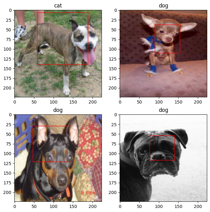
10 模型保存与预测
PATH = 'model_path/location_model.pth'
torch.save(model.state_dict(), PATH)
model = Net()
model.load_state_dict(torch.load(PATH))
model = model.cuda()        #.cpu() 模型使用GPU或CPU加载plt.figure(figsize=(8, 8))
imgs, _,_ = next(iter(test_dl))
imgs =imgs.to(device)
out1,out2 = model(imgs)
for i in range(4):plt.subplot(2, 2, i+1)plt.imshow(imgs[i].permute(1,2,0).detach().cpu())plt.title(id_to_name.get(torch.argmax(out2[i],0).item()))xmin, ymin, xmax, ymax = tuple(out1[i].detach().cpu().numpy()*224)rect = Rectangle((xmin, ymin), (xmax-xmin), (ymax-ymin), fill=False, color='red')ax = plt.gca()ax.axes.add_patch(rect)
plt.savefig('pics/predict.jpg',dpi =400)