来源：《斯坦福数据挖掘教程·第三版》对应的公开英文书和PPT。

Chapter 10 Mining Social-Network Graphs

The essential characteristics of a social network are:

1. There is a collection of entities that participate in the network. Typically, these entities are people, but they could be something else entirely.
2. There is at least one relationship between entities of the network. On Facebook or its ilk, this relationship is called friends. Sometimes the relationship is all-or-nothing; two people are either friends or they are not. However, in other examples of social networks, the relationship has a degree. This degree could be discrete; e.g., friends, family, acquaintances,
   or none as in Google+. It could be a real number; an example would be the fraction of the average day that two people spend talking to each other.
3. There is an assumption of nonrandomness or locality. This condition is the hardest to formalize, but the intuition is that relationships tend to cluster. That is, if entity A is related to both B and C, then there is a higher probability than average that B and C are related.

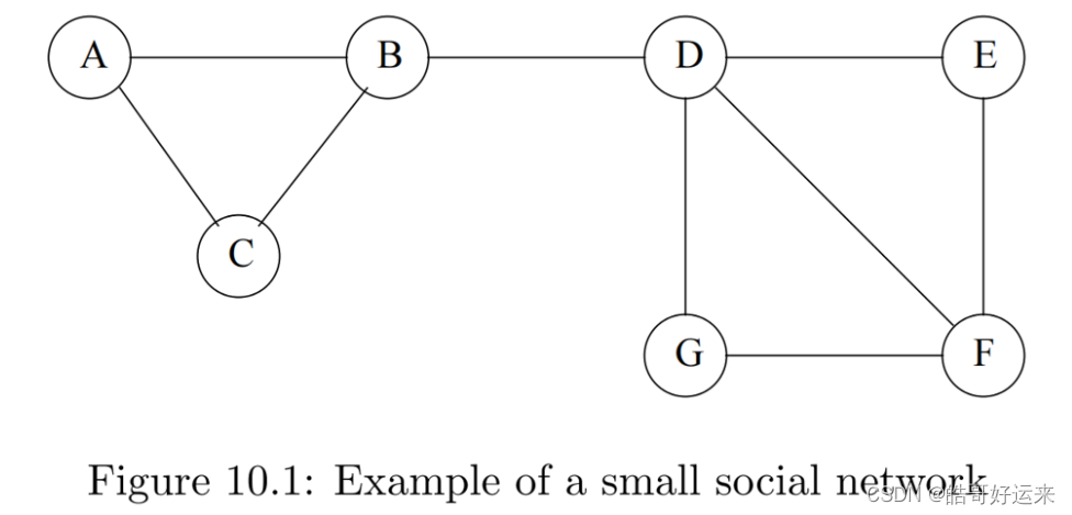
Social networks are naturally modeled as graphs, which we sometimes refer to as a social graph. The entities are the nodes, and an edge connects two nodes if the nodes are related by the relationship that characterizes the network. If there is a degree associated with the relationship, this degree is represented by labeling the edges. Often, social graphs are undirected, as for the Facebook friends graph. But they can be directed graphs, as for example the graphs of followers on Twitter or Google+.

There are many examples of social networks other than “friends” networks. Here, let us enumerate some of the other examples of networks that also exhibit locality of relationships.

Telephone Networks
Here the nodes represent phone numbers, which are really individuals. There is an edge between two nodes if a call has been placed between those phones in some fixed period of time, such as last month, or “ever.” The edges could be weighted by the number of calls made between these phones during the period. Communities in a telephone network will form from groups of people that communicate frequently: groups of friends, members of a club, or people working at the same company, for example.

Email Networks
The nodes represent email addresses, which are again individuals. An edge represents the fact that there was at least one email in at least one direction between the two addresses. Alternatively, we may only place an edge if there were emails in both directions. In that way, we avoid viewing spammers as “friends” with all their victims. Another approach is to label edges as weak or strong. Strong edges represent communication in both directions, while weak edges indicate that the communication was in one direction only. The communities seen in email networks come from the same sorts of groupings we mentioned in connection with telephone networks. A similar sort of network involves people who text other people through their cell phones.

Collaboration Networks
Nodes represent individuals who have published research papers. There is an edge between two individuals who published one or more papers jointly. Optionally, we can label edges by the number of joint publications. The communities in this network are authors working on a particular topic.
An alternative view of the same data is as a graph in which the nodes are papers. Two papers are connected by an edge if they have at least one author in common. Now, we form communities that are collections of papers on the same topic.
There are several other kinds of data that form two networks in a similar way. For example, we can look at the people who edit Wikipedia articles and the articles that they edit. Two editors are connected if they have edited an article in common. The communities are groups of editors that are interested in the same subject. Dually, we can build a network of articles, and connect
articles if they have been edited by the same person. Here, we get communities of articles on similar or related subjects.
In fact, the data involved in Collaborative filtering, as was discussed in Chapter 9, often can be viewed as forming a pair of networks, one for the customers and one for the products. Customers who buy the same sorts of products, e.g., science-fiction books, will form communities, and dually, products that are bought by the same customers will form communities, e.g., all science-fiction books.

Other Examples of Social Graphs
Many other phenomena give rise to graphs that look something like social graphs, especially exhibiting locality. Examples include: information networks (documents, web graphs, patents), infrastructure networks (roads, planes, water pipes, powergrids), biological networks (genes, proteins, food-webs of animals eating each other), as well as other types, like product co-purchasing networks (e.g., Groupon).

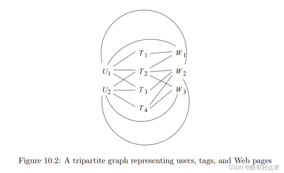
Figure 10.2 is an example of a tripartite graph (the case k = 3 of a k-partite graph). There are three sets of nodes, which we may think of as users { U 1 , U 2 } \{U_1, U_2\} {U1​,U2​}, tags { T 1 , T 2 , T 3 , T 4 } \{T_1, T_2, T_3, T_4\} {T1​,T2​,T3​,T4​}, and Web pages { W 1 , W 2 , W 3 } \{W_1, W_2, W_3\} {W1​,W2​,W3​}.
Define the betweenness of an edge $(a,b)$ to be the number of pairs of nodes $x$ and $y$ such that the edge $(a,b)$ lies on the shortest path between $x$ and $y$. To be more precise, since there can be several shortest paths between $x$ and $y$, edge $(a,b)$ is credited with the fraction of those shortest paths that include the edge $(a,b)$. As in golf, a high score is bad. It suggests that the edge $(a,b)$ runs between two different communities; that is, $a$ and $b$ do not belong to the same community.

Following is Girvan-Newman Algorithm

Can see this blog: Girvan-Newman Algorithm

A proper definition of a “good” cut must balance the size of the cut itself against the difference in the sizes of the sets that the cut creates. One choice that serves well is the “normalized cut.” First, define the volume of a set S of nodes, denoted $Vol(S)$, to be the number of edges with at least one end in S. Suppose we partition the nodes of a graph into two disjoint sets S and T .
Let $Cut(S,T)$ be the number of edges that connect a node in S to a node in T . Then the normalized cut value for S and T is

$$\frac{Cut(S,T)}{Vol(S)}+\frac{Cut(S,T)}{Vol(T)}$$

Suppose our graph has adjacency matrix A and degree matrix D. Our third matrix, called the Laplacian matrix, is $L=D-A$, the difference between the degree matrix and the adjacency matrix. That is, the Laplacian matrix L has the same entries as D on the diagonal. Off the diagonal, at row i and column j, L has −1 if there is an edge between nodes i and j and 0 if not.

Eigenvalues of the Laplacian Matrix

The smallest eigenvalue for every Laplacian matrix is 0, and its corresponding eigenvector is [1, 1, . . . , 1].

There is a simple way to find the second-smallest eigenvalue for any matrix, such as the Laplacian matrix, that is symmetric (the entry in row $i$ and column
$j$ equals the entry in row $j$ and column $i$). While we shall not prove this fact, the second-smallest eigenvalue of L is the minimum of $x^{T}Lx$, where $x=[x_1,x_2,...,x_n]$ is a column vector with n components, and the minimum is
taken under the constraints:

1. The length of x is 1; that is ${\sum }_{i=1}^n{x}_i^2=1$
2. $x$ is orthogonal to the eigenvector associated with the smallest eigenvalue.

When L is a Laplacian matrix for an n-node graph, we know something more. The eigenvector associated with the smallest eigenvalue is 1. Thus, if x is orthogonal to 1, we must have

$${\mathbf{x}}^{T}1=\sum _{i=1}^n{x}_i=0$$

In addition for the Laplacian matrix, the expression $x^{T}Lx$ has a useful equivalent expression. Recall that $L=D-A$, where D and A are the degree and adjacency matrices of the same graph. Thus, $x^{T}Lx=x^{T}Dx-x^{T}Ax$.

The Affiliation-Graph Model

The elements of the graph-generation mechanism are:

1. There is a given number of communities, and there is a given number of individuals (nodes of the graph).
2. Each community can have any set of individuals as members. That is, the memberships in the communities are parameters of the model.
3. Each community C has a probability $p_C$ associated with it, the probability that two members of community C are connected by an edge because they are both members of C. These probabilities are also parameters of the model.
4. If a pair of nodes is in two or more communities, then there is an edge between them if any of the communities of which both are members induces that edge according to Rule (3).
5. The decision whether a community induces an edge between two of its members is independent of that decision for any other community of which these two individuals are also members.

There is a solution to the problem caused by the affiliation-graph model, where membership of individuals in communities is discrete: either you are a member of the community or not. Instead of “all-or-nothing” membership of nodes in communities, we can suppose that for each node and each community, there is a “strength of membership” for that node and community. Intuitively, the stronger the membership of two individuals in the same community is, the more likely it is that this community will cause there to be an edge between them.

In this model, we can adjust the strength of membership for an individual in a community continuously, just as we can adjust the probability associated with a community in the affiliation-graph model. That improvement allows us to use methods for optimizing continuous functions, such as gradient descent, to maximize the expression for likelihood. In the new model, we have

1. Fixed sets of communities and individuals, as before.

2. For each community C and individual x, there is a strength of membership
   parameter $F_{xC}$ . These parameters can take any nonnegative value, and a value of 0 means the individual is definitely not in the community.

3. The probability that community C causes there to be an edge between nodes u and v is

   $$p_C(u,v)=1-e^{-F_{uC}{F}_{vC}}$$

As before, the probability of there being an edge between u and v is 1 minus the probability that none of the communities causes there to be an edge between them. That is, each community independently causes edges, and an edge exists between two nodes if any community causes it to exist. More formally, $p_{uv}$, the probability of an edge between nodes u and v, is

$$p_{uv}=1-\prod _C(1-p_C(u,v))$$

Finally, let E be the set of edges in the observed graph. As before, we can write the formula for the likelihood of the observed graph as the product of the expression for $p_{uv}$ for each edge $(u,v)$ that is in E, times the product of $1-p_{uv}$ for each edge $(u,v)$ that is not in E. Thus, in the new model, the formula for the likelihood of the graph with edges E is

$$\prod _{(u,v)inE}(1-e^{-F_{uC}{F}_{vC}})\prod _{(u,v)notinE}(e^{-F_{uC}{F}_{vC}})$$

💡 Continuous Versus Discrete Optimization

Whenever you are trying to find an optimum solution to a problem where some of the elements are continuous (e.g., the probabilities of communities inducing edges) and some elements are discrete (e.g., the memberships of the communities), it might make sense to replace each discrete element by a continuous variable. That change, while it doesn’t strictly speaking represent reality, enables us to perform only one optimization, which will use a continuous optimization method such as gradient descent. We run the risk of winding up in a local optimum that is not the globally best solution.

SimRank

In this section, we shall take up another approach to analyzing social-network graphs. This technique, called “simrank,” applies best to graphs with several types of nodes, although it can in principle be applied to any graph. The purpose of simrank is to measure the similarity between nodes of the same type, and it does so by seeing where random walkers on the graph wind up when starting at a particular node, the source node. Because calculation must be carried out once for each source node, there is a limit to the size of graphs that can be analyzed completely in this manner. However, we shall also offer an algorithm that approximates simrank, but is far more efficient than iterated matrix-vector multiplication. Finally, we show how simrank can be used to find communities.

Let us use β as the probability that the walker continues at random, so 1 − β is the probability the walker will teleport to the source node S. Let $e_S$ be the column vector that has 1 in the row for node S and 0’s elsewhere. Then if v is the column vector that reflects the probability the walker is at each of the nodes at a particular round, and $v\prime$ is the probability the walker is at each of the nodes at the next round, then $v\prime$ is related to v by:

$$v^{\prime }=\beta Mv+(1-\beta )e_S$$

A simple approach is to add nodes until the density of edges – the fraction of edges that connect nodes in the community divided by the number of possible edges connecting nodes in the community (i.e.,$C_2^n$ for an n-node community) – goes below a threshold.

Another measure of the goodness of a community C is the conductance. To define conductance, we need first to define the volume of a community C, which is the smaller of the sum of the degrees of the nodes in C and the sum of the degrees of the nodes not in C. Then the conductance of C is the ratio of the number of edges with exactly one end in C divided by the volume of C. The intuitive idea behind conductance is that it looks for sets C that are neither too small nor too large, and yet can be disconnected from the network by cutting a relatively small number of edges. Small conductance suggests a closely knit community.

The neighborhood of radius d for a node v is the set of nodes u for which there is a path of length at most d from v to u. We denote this neighborhood by $N(v,d)$. For example, N(v, 0) is always {v}, and N(v, 1) is v plus the set of nodes to which there is an arc from v. More generally, if V is a set of nodes, then N(V, d) is the set of nodes u for which there is a path of length d or less from at least one node in the set V .

The neighborhood profile of a node v is the sequence of sizes of its neighborhoods $|N(v,1)|,|N(v,2)|,....$ We do not include the neighborhood of distance 0, since its size is always 1.

Summary of Chapter 10

• Social-Network Graphs: Graphs that represent the connections in a social network are not only large, but they exhibit a form of locality, where small subsets of nodes (communities) have a much higher density of edges than the average density.
• Communities and Clusters: While communities resemble clusters in some ways, there are also significant differences. Individuals (nodes) normally belong to several communities, and the usual distance measures fail to represent closeness among nodes of a community. As a result, standard algorithms for finding clusters in data do not work well for community finding.
• Betweenness: One way to separate nodes into communities is to measure the betweenness of edges, which is the sum over all pairs of nodes of the fraction of shortest paths between those nodes that go through the given edge. Communities are formed by deleting the edges whose betweenness is above a given threshold.
• The Girvan-Newman Algorithm: The Girvan-Newman Algorithm is an efficient technique for computing the betweenness of edges. A breadth-first search from each node is performed, and a sequence of labeling steps computes the share of paths from the root to each other node that go through each of the edges. The shares for an edge that are computed for each root are summed to get the betweenness.
• Communities and Complete Bipartite Graphs: A complete bipartite graph has two groups of nodes, all possible edges between pairs of nodes chosen one from each group, and no edges between nodes of the same group. Any sufficiently dense community (a set of nodes with many edges among them) will have a large complete bipartite graph.
• Finding Complete Bipartite Graphs: We can find complete bipartite graphs by the same techniques we used for finding frequent itemsets. Nodes of the graph can be thought of both as the items and as the baskets. The basket corresponding to a node is the set of adjacent nodes, thought of as items. A complete bipartite graph with node groups of size t and s can be thought of as finding frequent itemsets of size t with supports.
• Graph Partitioning: One way to find communities is to partition a graph repeatedly into pieces of roughly similar sizes. A cut is a partition of the nodes of the graph into two sets, and its size is the number of edges that have one end in each set. The volume of a set of nodes is the number of edges with at least one end in that set.
• Normalized Cuts: We can normalize the size of a cut by taking the ratio of the size of the cut and the volume of each of the two sets formed by the cut. Then add these two ratios to get the normalized cut value. Normalized cuts with a low sum are good, in the sense that they tend to divide the nodes into two roughly equal parts, and have a relatively small size.
• Adjacency Matrices: These matrices describe a graph. The entry in row i and column j is 1 if there is an edge between nodes i and j, and 0 otherwise.
• Degree Matrices: The degree matrix for a graph has d in the ith diagonal entry if d is the degree of the ith node. Off the diagonal, all entries are 0.
• Laplacian Matrices: The Laplacian matrix for a graph is its degree matrix minus its adjacency matrix. That is, the entry in row i and column i of the Laplacian matrix is the degree of the ith node of the graph, and the entry in row i and column j, for i 6 = j, is −1 if there is an edge between nodes i and j, and 0 otherwise.
• Spectral Method for Partitioning Graphs: The lowest eigenvalue for any Laplacian matrix is 0, and its corresponding eigenvector consists of all 1’s. The eigenvectors corresponding to small eigenvalues can be used to guide a partition of the graph into two parts of similar size with a small cut value. For one example, putting the nodes with a positive component in the eigenvector with the second-smallest eigenvalue into one set and those with a negative component into the other is usually good.
• Overlapping Communities: Typically, individuals are members of several communities. In graphs describing social networks, it is normal for the probability that two individuals are friends to rise as the number of communities of which both are members grows.
• The Affiliation-Graph Model: An appropriate model for membership in communities is to assume that for each community there is a probability that because of this community two members become friends (have an edge in the social network graph). Thus, the probability that two nodes have an edge is 1 minus the product of the probabilities that none of the communities of which both are members cause there to be an edge between them. We then find the assignment of nodes to communities and the values of those probabilities that best describes the observed social graph.
• Maximum-Likelihood Estimation: An important modeling technique, useful for modeling communities as well as many other things, is to compute, as a function of all choices of parameter values that the model allows, the probability that the observed data would be generated. The values that yield the highest probability are assumed to be correct, and called the maximum-likelihood estimate (MLE).
• Use of Gradient Descent: If we know membership in communities, we can find the MLE by gradient descent or other methods. However, we cannot find the best membership in communities by gradient descent, because membership is discrete, not continuous.
• Improved Community Modeling by Strength of Membership: We can formulate the problem of finding the MLE of communities in a social graph by assuming individuals have a strength of membership in each community, possibly 0 if they are not a member. If we define the probability of an edge between two nodes to be a function of their membership strengths in their common communities, we can turn the problem of finding the MLE into a continuous problem and solve it using gradient descent.
• Simrank: One way to measure the similarity of nodes in a graph with several types of nodes is to start a random walker at one node and allow it to wander, with a fixed probability of restarting at the same node. The distribution of where the walker can be expected to be is a good measure of the similarity of nodes to the starting node. This process must be repeated with each node as the starting node if we are to get all-pairs similarity.
• Triangles in Social Networks: The number of triangles per node is an important measure of the closeness of a community and often reflects its maturity. We can enumerate or count the triangles in a graph with m edges in $O(m^{3/2})$ time, but no more efficient algorithm exists in general.
• Triangle Finding by MapReduce: We can find triangles in a single round of MapReduce by treating it as a three-way join. Each edge must be sent to a number of reducers proportional to the cube root of the total number of reducers, and the total computation time spent at all the reducers is proportional to the time of the serial algorithm for triangle finding.
• Neighborhoods: The neighborhood of radius d for a node v in a directed or undirected graph is the set of nodes reachable from v along paths of length at most d. The neighborhood profile of a node is the sequence of neighborhood sizes for all distances from 1 upwards. The diameter of a connected graph is the smallest d for which the neighborhood of radius d for any starting node includes the entire graph.
• Transitive Closure: A node v can reach node u if u is in the neighborhood of v for some radius. The transitive closure of a graph is the set of pairs of nodes (v, u) such that v can reach u.
• Computing Transitive Closure: Since the transitive closure can have a number of facts equal to the square of the number of nodes of a graph, it is infeasible to compute transitive closure directly for large graphs. One approach is to find strongly connected components of the graph and collapse them each to a single node before computing the transitive closure.
• Transitive Closure and MapReduce: We can view transitive closure computation as the iterative join of a path relation (pairs of nodes v and u such that u is known to be reachable from v) and the arc relation of the graph. Such an approach requires a number of MapReduce rounds equal to the diameter of the graph.
• Seminaive Evaluation: When computing the transitive closure for a graph, we can speed up the iterative evaluation of the Path relation by recognizing that a Path fact is only useful on the round after that round when it was first discovered. A similar idea speeds up the reachability calculation and many similar iterative algorithms.
• Transitive Closure by Recursive Doubling: An approach that uses fewer MapReduce rounds is to join the path relation with itself at each round. At each round, we double the length of paths that are able to contribute to the transitive closure. Thus, the number of needed rounds is only the base-2 logarithm of the diameter of the graph.
• Smart Transitive Closure: While recursive doubling can cause the same path to be considered many times, and thus increases the total computation time (compared with iteratively joining paths with single arcs), a variant called smart transitive closure avoids discovering the same path more than once. The trick is to require that when joining two paths, the first has a length that is a power of 2.
• Approximating Neighborhood Sizes: By using the Flajolet-Martin technique for approximating the number of distinct elements in a stream, we can find the neighborhood sizes at different radii approximately. We maintain a set of tail lengths for each node. To increase the radius by 1, we examine each edge (u, v) and for each tail length for u we set it equal to the corresponding tail length for v if the latter is larger than the former.