文章目录
- 因子分析
- 数据集
- 处理步骤
- 主成分法做因子分析
- 最大似然法做因子分析
因子分析
-
因子分析的用途与主成分分析类似,它也是一种降维方法。由于因子往往比主成分更易得到解释,故因子分析比主成分分析更容易成功,从而有更广泛的应用。
-
从方法上来说,因子分析比主成分分析更为精细,自然理论上也就更为复杂。主成分分析只涉及一般的线性变换,不涉及模型,仅需假定二阶矩存在。而因子分析需建立一个数学模型,并作一定的假定。
-
因子分析起源于20世纪初,K.皮尔逊(
Pearson)和C.斯皮尔曼(Spearman)等学者为定义和测定智力所作的努力,主要是由对心理测量学有兴趣的科学家们培育和发展了因子分析。 -
因子分析的目的是为了
降维,降维的方式是试图用少数几个潜在的、不可观测的随机变量来描述原始变量间的协方差关系。
数据集
内置的mtcars数据框包含有关32辆汽车的信息,包括它们的重量,燃油效率(以每加仑英里为单位),速度等。
数据来自1974年美国汽车趋势杂志,包括32辆汽车(1973-74款)的油耗和10个方面的汽车设计和性能。
> help("mtcars")Motor Trend Car Road Tests
Description
The data was extracted from the 1974 Motor Trend US magazine, and comprises fuel consumption and 10 aspects of automobile design and performance for 32 automobiles (1973–74 models).Usage
mtcars
Format
A data frame with 32 observations on 11 (numeric) variables.[, 1]	mpg	Miles/(US) gallon
[, 2]	cyl	Number of cylinders
[, 3]	disp	Displacement (cu.in.)
[, 4]	hp	Gross horsepower
[, 5]	drat	Rear axle ratio
[, 6]	wt	Weight (1000 lbs)
[, 7]	qsec	1/4 mile time
[, 8]	vs	Engine (0 = V-shaped, 1 = straight)
[, 9]	am	Transmission (0 = automatic, 1 = manual)
[,10]	gear	Number of forward gears
[,11]	carb	Number of carburetors
Source
Henderson and Velleman (1981), Building multiple regression models interactively. Biometrics, 37, 391–411.Examples
require(graphics)
pairs(mtcars, main = "mtcars data", gap = 1/4)
coplot(mpg ~ disp | as.factor(cyl), data = mtcars,panel = panel.smooth, rows = 1)
## possibly more meaningful, e.g., for summary() or bivariate plots:
mtcars2 <- within(mtcars, {vs <- factor(vs, labels = c("V", "S"))am <- factor(am, labels = c("automatic", "manual"))cyl  <- ordered(cyl)gear <- ordered(gear)carb <- ordered(carb)
})
summary(mtcars2)
处理步骤
- 根据研究的问题选取原始变量
- 对原始变量进行标准化并求出相关阵,分析变量之间的相关性
- 求解初始公因子及其因子载荷矩阵
- 因子旋转
- 计算因子得分
- 绘制因子载荷图,因子得分图
主成分法做因子分析
- 不做因子旋转,使用原始数据
因子数选择为3个
library("psych")fac<-principal(mtcars,3,rotate="none")
fac
- 不做因子旋转,使用相关系数矩阵
有些题目直接给出相关系数矩阵,没有原始数据,也可以使用因子分析的主成分法,得到的结果相同
Standardized loadings:标准化后的载荷矩阵
Principal Components Analysis
Call: principal(r = R, nfactors = 3, rotate = "none")
Standardized loadings (pattern matrix) based upon correlation matrixPC1   PC2   PC3   h2    u2 com
mpg  -0.93  0.03 -0.18 0.90 0.099 1.1
cyl   0.96  0.07 -0.14 0.95 0.052 1.1
disp  0.95 -0.08 -0.05 0.90 0.095 1.0
hp    0.85  0.41  0.11 0.90 0.104 1.5
drat -0.76  0.45  0.13 0.79 0.212 1.7
wt    0.89 -0.23  0.27 0.92 0.081 1.3
qsec -0.52 -0.75  0.32 0.94 0.063 2.2
vs   -0.79 -0.38  0.34 0.88 0.122 1.8
am   -0.60  0.70 -0.16 0.88 0.120 2.1
gear -0.53  0.75  0.23 0.90 0.098 2.0
carb  0.55  0.67  0.42 0.93 0.069 2.6PC1  PC2  PC3
SS loadings           6.61 2.65 0.63
Proportion Var        0.60 0.24 0.06
Cumulative Var        0.60 0.84 0.90
Proportion Explained  0.67 0.27 0.06
Cumulative Proportion 0.67 0.94 1.00Mean item complexity =  1.7
Test of the hypothesis that 3 components are sufficient.The root mean square of the residuals (RMSR) is  0.03 Fit based upon off diagonal values = 1
从累积方差贡献率来看,取3个因子的累积方差贡献率为90%,取两个因子的累积方差贡献率为84%。
因此我们可以将因子数减少到两个,有利于可视化分析。
fac<-principal(mtcars,2,rotate="none")
facPrincipal Components Analysis
Call: principal(r = mtcars, nfactors = 2, rotate = "none")
Standardized loadings (pattern matrix) based upon correlation matrixPC1   PC2   h2    u2 com
mpg  -0.93  0.03 0.87 0.131 1.0
cyl   0.96  0.07 0.93 0.071 1.0
disp  0.95 -0.08 0.90 0.098 1.0
hp    0.85  0.41 0.88 0.116 1.4
drat -0.76  0.45 0.77 0.228 1.6
wt    0.89 -0.23 0.85 0.154 1.1
qsec -0.52 -0.75 0.83 0.165 1.8
vs   -0.79 -0.38 0.76 0.237 1.4
am   -0.60  0.70 0.85 0.146 2.0
gear -0.53  0.75 0.85 0.150 1.8
carb  0.55  0.67 0.76 0.244 1.9PC1  PC2
SS loadings           6.61 2.65
Proportion Var        0.60 0.24
Cumulative Var        0.60 0.84
Proportion Explained  0.71 0.29
Cumulative Proportion 0.71 1.00Mean item complexity =  1.5
Test of the hypothesis that 2 components are sufficient.The root mean square of the residuals (RMSR) is  0.05 with the empirical chi square  9.45  with prob <  1 Fit based upon off diagonal values = 0.99
可以发现,因子数从3个减少到2个时,使用主成分法,前两个主成分的方差贡献率不会变化。这跟最大似然法不同。
- 绘制因子载荷图
#绘制因子载荷图
plot(fac1$loadings,xlab="Factor1",ylab="Factor2")
abline(h=0);abline(v=0)
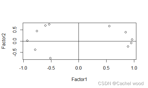
可以发现很多点离两个因子都比较远,不好解释。
- 主成分法,使用最大方差法进行因子旋转
因子数选择为2,并计算因子得分
> #主成分法,方差最大化做因子正交旋转
> fac2<-principal(mtcars,2,rotate="varimax")
> fac2
Principal Components Analysis
Call: principal(r = mtcars, nfactors = 2, rotate = "varimax")
Standardized loadings (pattern matrix) based upon correlation matrixRC1   RC2   h2    u2 com
mpg   0.68 -0.63 0.87 0.131 2.0
cyl  -0.64  0.72 0.93 0.071 2.0
disp -0.73  0.60 0.90 0.098 1.9
hp   -0.32  0.88 0.88 0.116 1.3
drat  0.85 -0.21 0.77 0.228 1.1
wt   -0.80  0.46 0.85 0.154 1.6
qsec -0.16 -0.90 0.83 0.165 1.1
vs    0.30 -0.82 0.76 0.237 1.3
am    0.92  0.08 0.85 0.146 1.0
gear  0.91  0.17 0.85 0.150 1.1
carb  0.08  0.87 0.76 0.244 1.0RC1  RC2
SS loadings           4.67 4.59
Proportion Var        0.42 0.42
Cumulative Var        0.42 0.84
Proportion Explained  0.50 0.50
Cumulative Proportion 0.50 1.00Mean item complexity =  1.4
Test of the hypothesis that 2 components are sufficient.The root mean square of the residuals (RMSR) is  0.05 with the empirical chi square  9.45  with prob <  1 Fit based upon off diagonal values = 0.99> #计算因子得分
> fac2$scoresRC1        RC2
Mazda RX4            0.913545261  0.5740734
Mazda RX4 Wag        0.827547997  0.5013891
Datsun 710           0.698816380 -0.8074274
Hornet 4 Drive      -0.913638812 -1.1047271
Hornet Sportabout   -0.859350144  0.2025926
Valiant             -1.162422544 -1.2190911
Duster 360          -0.680268641  0.9486423
Merc 240D           -0.056857408 -1.1835017
Merc 230            -0.212468151 -1.4696568
Merc 280             0.075581300 -0.2109478
Merc 280C            0.002444315 -0.2763119
Merc 450SE          -0.904174186  0.3064233
Merc 450SL          -0.849329738  0.2529898
Merc 450SLC         -0.927001103  0.2287337
Cadillac Fleetwood  -1.417403948  0.6862707
Lincoln Continental -1.392296773  0.7416873
Chrysler Imperial   -1.161445427  0.7799435
Fiat 128             0.930026590 -1.1606987
Honda Civic          1.455372982 -0.8414166
Toyota Corolla       1.040852468 -1.2543364
Toyota Corona       -0.374988630 -1.4259630
Dodge Challenger    -1.026764303  0.1466255
AMC Javelin         -0.893224853  0.1071275
Camaro Z28          -0.502907752  1.0677154
Pontiac Firebird    -0.984122353  0.2236560
Fiat X1-9            0.926969145 -1.0092451
Porsche 914-2        1.590766193  0.1745827
Lotus Europa         1.509486177 -0.3106522
Ford Pantera L       1.103849172  1.8802235
Ferrari Dino         1.361140948  1.3909629
Maserati Bora        1.120968759  2.6074298
Volvo 142E           0.761297080 -0.5470932
>
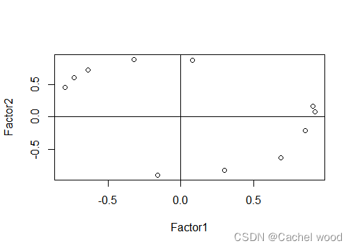
因子旋转之后,每个变量在某个因子上的载荷接近正负1,而在另一个因子上的载荷接近0,有助于我们进行解释分析。
- 绘制新的因子载荷图
#绘制因子载荷图
plot(fac2$loadings,xlab="Factor1",ylab="Factor2")
abline(h=0);abline(v=0)
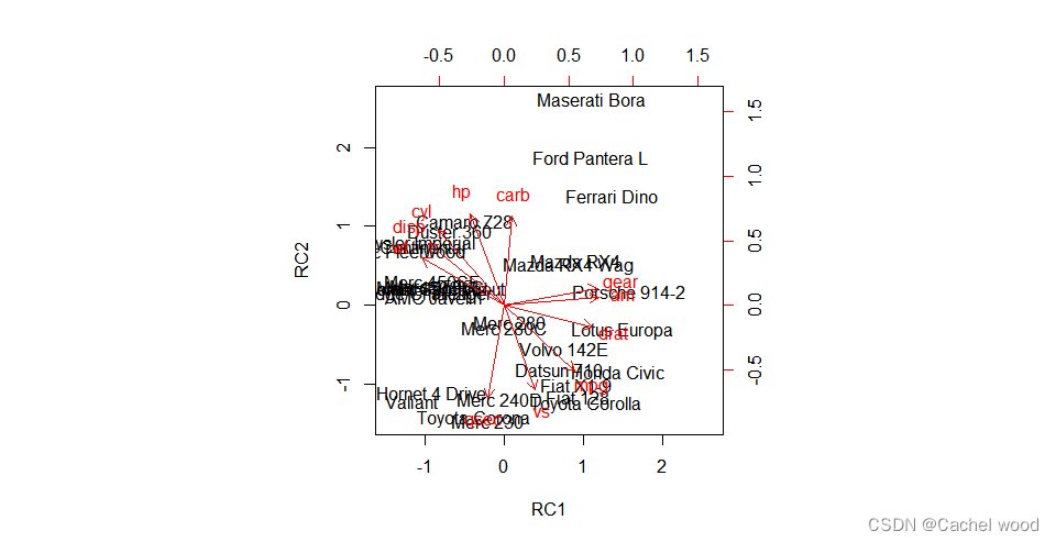
- 绘制因子得分图
#绘制每个学生的因子得分图与原坐标在因子上的方向,反应因子与原始数据的关系
biplot(fac2$scores,fac2$loadings)
- 主成分法分析
| 因子数 | 有无因子旋转 | 因子1方差贡献率 | 因子1方差贡献率 | 两因子累积贡献率 |
|---|---|---|---|---|
| 因子数为2 | 无因子旋转 | 60% | 24% | 84% |
| 因子数为2 | 有因子旋转 | 42% | 42% | 84% |
| 因子数为3 | 无因子旋转 | 60% | 24% | 84% |
| 因子数为3 | 有因子旋转 | 41% | 29% | 70% |
结论1:进行因子旋转会改变各因子的方差贡献率,但不会改变总方差贡献率
结论2:因子数不同,不进行因子旋转时,因子的方差贡献率不变
最大似然法做因子分析
- 不做因子旋转
#用极大似然法做因子分析
factanal(mtcars,factors = 2,rotation = "none")Call:
factanal(x = mtcars, factors = 2, rotation = "none")Uniquenesses:mpg   cyl  disp    hp  drat    wt  qsec    vs    am
0.167 0.070 0.096 0.143 0.298 0.168 0.150 0.256 0.171 gear  carb
0.246 0.386 Loadings:Factor1 Factor2
mpg  -0.910
cyl   0.962
disp  0.946
hp    0.851   0.364
drat -0.726   0.418
wt    0.867  -0.283
qsec -0.533  -0.752
vs   -0.783  -0.362
am   -0.578   0.703
gear -0.514   0.700
carb  0.537   0.571 Factor1 Factor2
SS loadings      6.439   2.412
Proportion Var   0.585   0.219
Cumulative Var   0.585   0.805Test of the hypothesis that 2 factors are sufficient.
The chi square statistic is 68.57 on 34 degrees of freedom.
The p-value is 0.000405
相对来说,因子载荷矩阵中,各变量在第一个因子上的载荷都比较大,不好解释,需要进行因子旋转。
前两个因子的累积方差解释率达到80.5%,满足要求。
- 进行因子旋转
> factanal(mtcars,factors = 2,rotation = "varimax")Call:
factanal(x = mtcars, factors = 2, rotation = "varimax")Uniquenesses:mpg   cyl  disp    hp  drat    wt  qsec    vs    am
0.167 0.070 0.096 0.143 0.298 0.168 0.150 0.256 0.171 gear  carb
0.246 0.386 Loadings:Factor1 Factor2
mpg   0.686  -0.602
cyl  -0.629   0.731
disp -0.730   0.609
hp   -0.337   0.862
drat  0.807  -0.225
wt   -0.810   0.420
qsec -0.162  -0.908
vs    0.291  -0.812
am    0.907
gear  0.860   0.125
carb          0.783 Factor1 Factor2
SS loadings      4.494   4.357
Proportion Var   0.409   0.396
Cumulative Var   0.409   0.805Test of the hypothesis that 2 factors are sufficient.
The chi square statistic is 68.57 on 34 degrees of freedom.
The p-value is 0.000405
- 因子数取3
> factanal(mtcars,factors = 3,rotation = "none")Call:
factanal(x = mtcars, factors = 3, rotation = "none")Uniquenesses:mpg   cyl  disp    hp  drat    wt  qsec    vs    am
0.135 0.055 0.090 0.127 0.290 0.060 0.051 0.223 0.208 gear  carb
0.125 0.158 Loadings:Factor1 Factor2 Factor3
mpg  -0.910   0.137  -0.136
cyl   0.962          -0.135
disp  0.937  -0.174
hp    0.875   0.292   0.147
drat -0.689   0.453   0.175
wt    0.858  -0.382   0.242
qsec -0.591  -0.754   0.177
vs   -0.809  -0.309   0.164
am   -0.522   0.719
gear -0.459   0.729   0.365
carb  0.594   0.517   0.471 Factor1 Factor2 Factor3
SS loadings      6.448   2.465   0.565
Proportion Var   0.586   0.224   0.051
Cumulative Var   0.586   0.810   0.862Test of the hypothesis that 3 factors are sufficient.
The chi square statistic is 30.53 on 25 degrees of freedom.
The p-value is 0.205
此时可以发现,最大似然法在改变因子个数时,不同因子的方差贡献率发生改变(虽然改变很小),其中因子1达到58.6%,因子2达到22.4%,前两个因子累积方差贡献率为81%。
- 因子数取3,进行因子旋转
对极大似然解,当因子数增加时,原来因子的估计载荷及对x的贡献将发生变化,这与主成分解不同。因子数可由主成分法初步确定。
> factanal(mtcars,factors = 3,rotation = "varimax")Call:
factanal(x = mtcars, factors = 3, rotation = "varimax")Uniquenesses:mpg   cyl  disp    hp  drat    wt  qsec    vs    am
0.135 0.055 0.090 0.127 0.290 0.060 0.051 0.223 0.208 gear  carb
0.125 0.158 Loadings:Factor1 Factor2 Factor3
mpg   0.643  -0.478  -0.473
cyl  -0.618   0.703   0.261
disp -0.719   0.537   0.323
hp   -0.291   0.725   0.513
drat  0.804  -0.241
wt   -0.778   0.248   0.524
qsec -0.177  -0.946  -0.151
vs    0.295  -0.805  -0.204
am    0.880
gear  0.908           0.224
carb  0.114   0.559   0.719 Factor1 Factor2 Factor3
SS loadings      4.380   3.520   1.578
Proportion Var   0.398   0.320   0.143
Cumulative Var   0.398   0.718   0.862Test of the hypothesis that 3 factors are sufficient.
The chi square statistic is 30.53 on 25 degrees of freedom.
The p-value is 0.205
因子数取3,进行因子旋转之后,因子1的方差解释率下降到39.8%,前两个因子累积贡献率达到71.8%,发生变化。
- 最大似然法分析
| 因子数 | 有无因子旋转 | 因子1方差贡献率 | 因子1方差贡献率 | 两因子累积贡献率 |
|---|---|---|---|---|
| 因子数为2 | 无因子旋转 | 58.5% | 21.9% | 80.5% |
| 因子数为2 | 有因子旋转 | 40.9% | 39.6% | 80.5% |
| 因子数为3 | 无因子旋转 | 58.6% | 22.4% | 81% |
| 因子数为3 | 有因子旋转 | 39.8% | 32% | 71.8% |
结论1:进行因子旋转会改变各因子的方差贡献率以及总方差贡献率
结论2:因子数不同也会改变各因子的方差贡献率


![[云原生1.]Docker数据管理与Cgroups资源控制管理](https://img-blog.csdnimg.cn/08c1c69e17064a4dac29d5306451f21c.png)