文章目录
- 概要
- 前置条件
- 统计数据分析
- 直方图均衡化原理
- 小结
概要
图像处理是计算机视觉领域中的重要组成部分,而直方图在图像处理中扮演着关键的角色。如何巧妙地运用OpenCV库中的图像处理技巧,特别是直方图相关的方法,来提高图像质量、改善细节以及调整曝光。
通过对图像的直方图进行分析和调整,能够优化图像的对比度、亮度和色彩平衡,从而使图像更具可视化效果。
直方图是一种统计图,用于表示图像中像素灰度级别的分布情况。在OpenCV中,可以使用直方图来了解图像的整体亮度分布,从而为后续处理提供基础。
OpenCV库中的函数,如cv2.calcHist和cv2.equalizeHist等,对图像的直方图进行均衡化。直方图均衡化是一种有效的方法,通过重新分配像素的强度值,使图像的亮度分布更均匀,提高图像的对比度和细节。
直方图匹配的应用,通过将目标图像的直方图调整到参考图像的直方图,实现两者之间的色彩一致性。这在图像配准和合成中有广泛的应用,提高了图像处理的精度和效果。
在低光照条件下拍摄图像的处理技巧。通过分析图像的直方图,可以采取针对性的方法,提高低光照图像中物体的可见性,改善图像的细节,并校正曝光过度或曝光不足的问题。
前置条件
一般来说,通过合理利用一些直方图的技巧,可以用于提高低光照拍摄图像中物体的可见性,改善图像的细节,以及校正曝光过度或曝光不足的图像。
import numpy as np
import matplotlib.pyplot as plt
from skimage.color import rgb2gray
from skimage.exposure import histogram, cumulative_distribution
from skimage import filters
from skimage.color import rgb2hsv, rgb2gray, rgb2yuv
from skimage import color, exposure, transform
from skimage.exposure import histogram, cumulative_distributionfrom skimage.io import imread# Load the image & remove the alpha or opacity channel (transparency)
dark_image = imread('img.png')[:,:,:3]# Visualize the image
plt.figure(figsize=(10, 10))
plt.title('Original Image: Plasma Ball')
plt.imshow(dark_image)
plt.show()
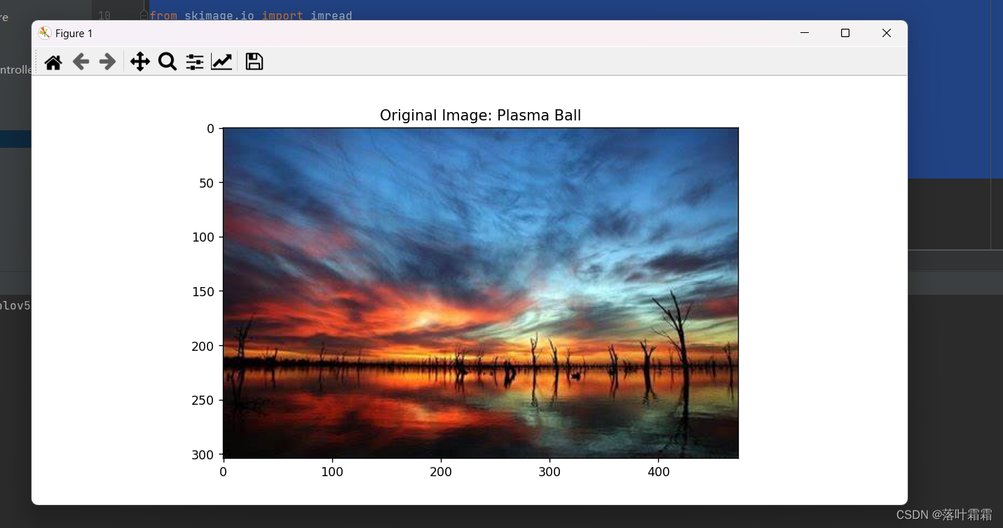
上述图像是在光照不足下进行拍摄的,接着我们就来通过控制直方图,来改善我们的视觉效果。
统计数据分析
使用以下代码:
def calc_color_overcast(image):# Calculate color overcast for each channelred_channel = image[:, :, 0]green_channel = image[:, :, 1]blue_channel = image[:, :, 2]# Create a dataframe to store the resultschannel_stats = pd.DataFrame(columns=['Mean', 'Std', 'Min', 'Median', 'P_80', 'P_90', 'P_99', 'Max'])# Compute and store the statistics for each color channelfor channel, name in zip([red_channel, green_channel, blue_channel], ['Red', 'Green', 'Blue']):mean = np.mean(channel)std = np.std(channel)minimum = np.min(channel)median = np.median(channel)p_80 = np.percentile(channel, 80)p_90 = np.percentile(channel, 90)p_99 = np.percentile(channel, 99)maximum = np.max(channel)channel_stats.loc[name] = [mean, std, minimum, median, p_80, p_90, p_99, maximum]return channel_stats
完整代码:
import numpy as np
import matplotlib.pyplot as plt
from skimage.color import rgb2gray
from skimage.exposure import histogram, cumulative_distribution
from skimage import filters
from skimage.color import rgb2hsv, rgb2gray, rgb2yuv
from skimage import color, exposure, transform
from skimage.exposure import histogram, cumulative_distribution
import pandas as pdfrom skimage.io import imread# Load the image & remove the alpha or opacity channel (transparency)
dark_image = imread('img.png')[:,:,:3]# Visualize the image
plt.figure(figsize=(10, 10))
plt.title('Original Image: Plasma Ball')
plt.imshow(dark_image)
plt.show()def calc_color_overcast(image):# Calculate color overcast for each channelred_channel = image[:, :, 0]green_channel = image[:, :, 1]blue_channel = image[:, :, 2]# Create a dataframe to store the resultschannel_stats = pd.DataFrame(columns=['Mean', 'Std', 'Min', 'Median','P_80', 'P_90', 'P_99', 'Max'])# Compute and store the statistics for each color channelfor channel, name in zip([red_channel, green_channel, blue_channel],['Red', 'Green', 'Blue']):mean = np.mean(channel)std = np.std(channel)minimum = np.min(channel)median = np.median(channel)p_80 = np.percentile(channel, 80)p_90 = np.percentile(channel, 90)p_99 = np.percentile(channel, 99)maximum = np.max(channel)channel_stats.loc[name] = [mean, std, minimum, median, p_80, p_90, p_99, maximum]return channel_stats
# 调用函数并传入图像
result_stats = calc_color_overcast(dark_image)# 打印结果
print(result_stats)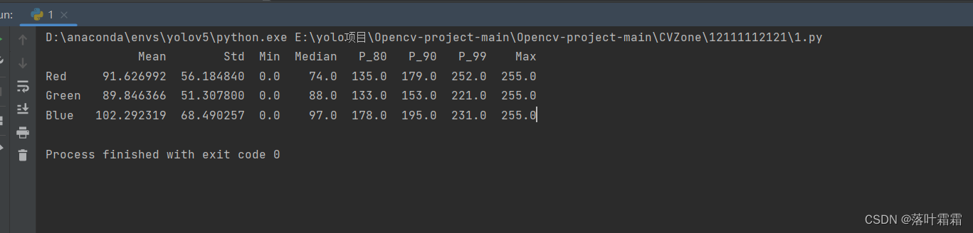
进而我们可以使用以下代码,来生成上述图像的直方图分布:
# Histogram plot
dark_image_intensity = img_as_ubyte(rgb2gray(dark_image))
freq, bins = histogram(dark_image_intensity)
plt.step(bins, freq*1.0/freq.sum())
plt.xlabel('intensity value')
plt.ylabel('fraction of pixels');
plt.show()  # 添加这一行以显示直方图
得到直方图可视化效果如下:
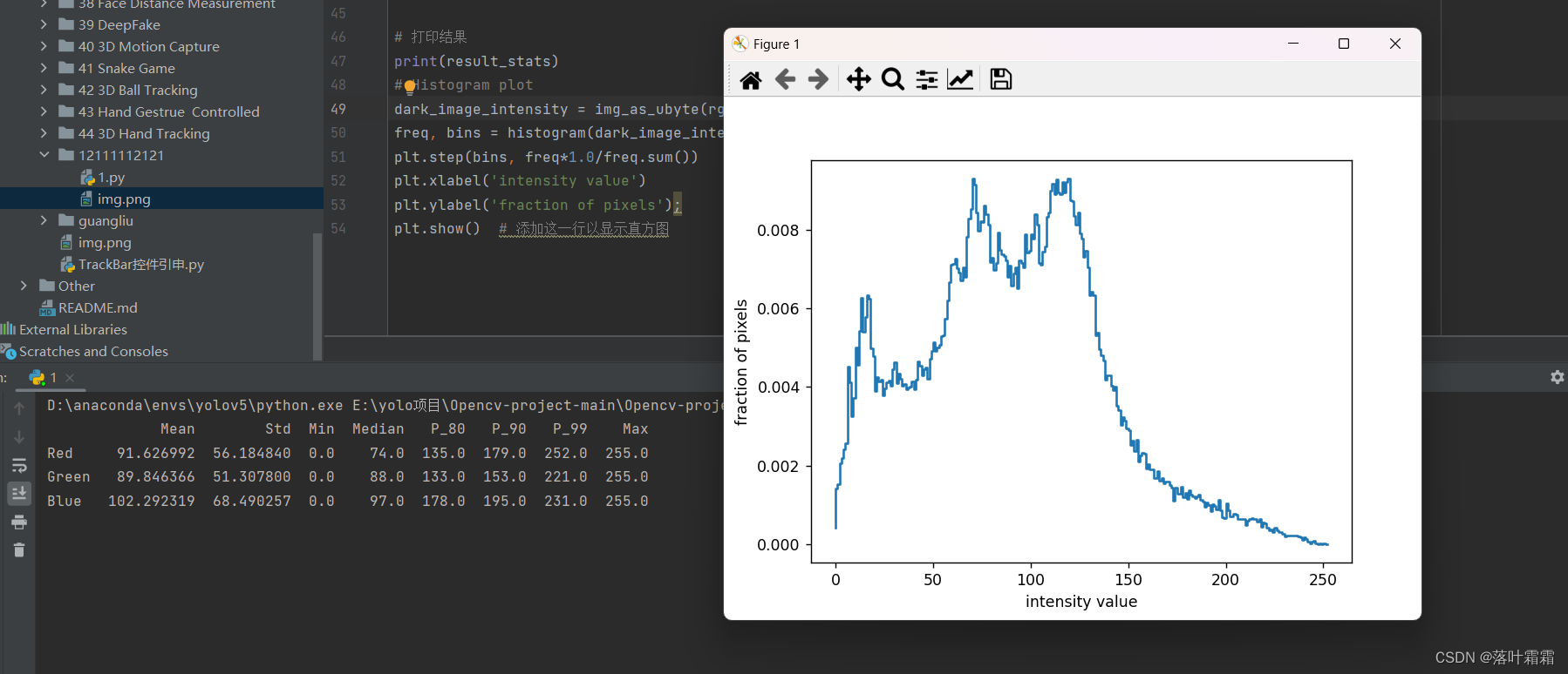
通过直方图的观察,可以注意到图像的像素平均强度似乎非常低,这进一步证实了图像的整体暗淡和曝光不足的情况。直方图展示了图像中像素强度值的分布情况,而大多数像素具有较低的强度值。这是有道理的,因为低像素强度值意味着图像中的大多数像素非常暗或呈现黑色。这样的观察有助于定量了解图像的亮度分布,为进一步的图像增强和调整提供了重要的线索。
直方图均衡化原理
直方图均衡化的基本原理是通过线性化图像的累积分布函数(CDF)来提高图像的对比度。实现这一目标的方法是将图像中每个像素的强度值映射到一个新的值,使得新的强度分布更加均匀。
可以通过以下几个步骤实现CDF的线性化:
将图像转换为灰度图:
如果图像不是灰度图,代码会将其转换为灰度图。这是因为直方图均衡化主要应用于灰度图。
计算累积分布函数(CDF):
通过计算图像像素的强度值的累积分布函数,可以了解每个强度值在图像中出现的累积频率。
绘制实际和目标CDF:
使用蓝色实线表示实际的CDF,使用红色实线表示目标CDF。目标CDF是一个线性分布,通过均匀分布来提高对比度。
绘制示例查找表:
绘制一个示例查找表,展示了像素强度值从原始值映射到目标值的过程。
自定义绘图:
对绘图进行自定义,包括设置坐标轴范围、标签和标题等。
import numpy as np
import matplotlib.pyplot as plt
from skimage.color import rgb2hsv, rgb2gray, rgb2yuv
from skimage.exposure import histogram, cumulative_distribution
import pandas as pd
from skimage import img_as_ubyte
from skimage.io import imread# Load the image & remove the alpha or opacity channel (transparency)
dark_image = imread('img.png')[:,:,:3]# Visualize the image
plt.figure(figsize=(10, 10))
plt.title('Original Image: Plasma Ball')
plt.imshow(dark_image)
plt.show()def calc_color_overcast(image):# Calculate color overcast for each channelred_channel = image[:, :, 0]green_channel = image[:, :, 1]blue_channel = image[:, :, 2]# Create a dataframe to store the resultschannel_stats = pd.DataFrame(columns=['Mean', 'Std', 'Min', 'Median','P_80', 'P_90', 'P_99', 'Max'])# Compute and store the statistics for each color channelfor channel, name in zip([red_channel, green_channel, blue_channel],['Red', 'Green', 'Blue']):mean = np.mean(channel)std = np.std(channel)minimum = np.min(channel)median = np.median(channel)p_80 = np.percentile(channel, 80)p_90 = np.percentile(channel, 90)p_99 = np.percentile(channel, 99)maximum = np.max(channel)channel_stats.loc[name] = [mean, std, minimum, median, p_80, p_90, p_99, maximum]return channel_statsdef plot_cdf(image):# Convert the image to grayscale if neededif len(image.shape) == 3:image = rgb2gray(image[:, :, :3])# Compute the cumulative distribution functionintensity = np.round(image * 255).astype(np.uint8)freq, bins = cumulative_distribution(intensity)# Plot the actual and target CDFstarget_bins = np.arange(256)target_freq = np.linspace(0, 1, len(target_bins))plt.step(bins, freq, c='b', label='Actual CDF')plt.plot(target_bins, target_freq, c='r', label='Target CDF')# Plot an example lookupexample_intensity = 50example_target = np.interp(freq[example_intensity], target_freq, target_bins)plt.plot([example_intensity, example_intensity, target_bins[-11], target_bins[-11]],[0, freq[example_intensity], freq[example_intensity], 0],'k--',label=f'Example lookup ({example_intensity} -> {example_target:.0f})')# Customize the plotplt.legend()plt.xlim(0, 255)plt.ylim(0, 1)plt.xlabel('Intensity Values')plt.ylabel('Cumulative Fraction of Pixels')plt.title('Cumulative Distribution Function')return freq, bins, target_freq, target_bins
# 调用函数并传入图像
result_stats = calc_color_overcast(dark_image)# 打印结果
print(result_stats)
# Histogram plot
# Histogram plot
dark_image_intensity = img_as_ubyte(rgb2gray(dark_image))
freq, bins = histogram(dark_image_intensity)
plt.step(bins, freq*1.0/freq.sum())
plt.xlabel('intensity value')
plt.ylabel('fraction of pixels')
plt.show()  # 添加这一行以显示直方图# 调用 plot_cdf 函数并传入图像
plot_cdf(dark_image)
plt.show()  # 添加这一行以显示CDF图形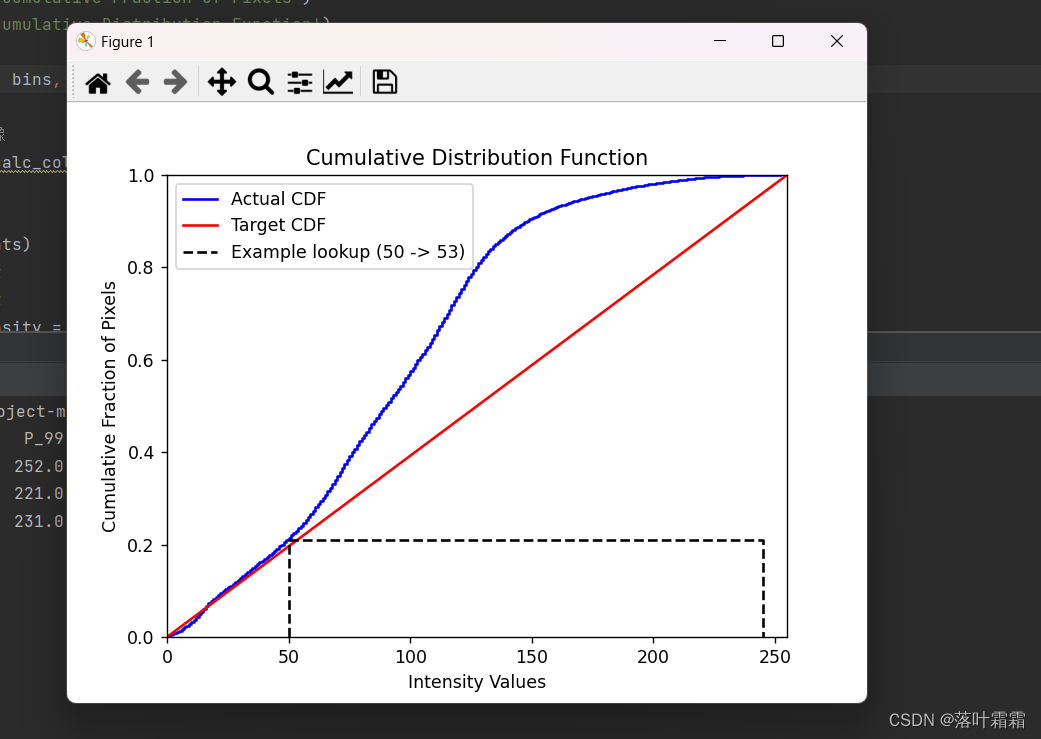
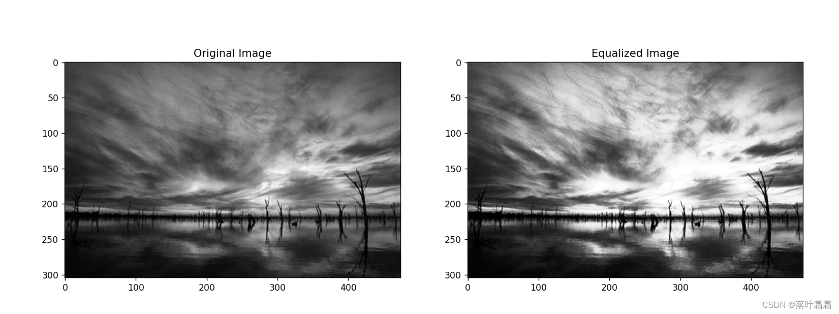
直方图均衡化实现结果:
import numpy as np
import matplotlib.pyplot as plt
from skimage.color import rgb2gray
from skimage.exposure import histogram, cumulative_distribution, equalize_hist
from skimage import img_as_ubyte
from skimage.io import imread# Load the image & remove the alpha or opacity channel (transparency)
dark_image = imread('img.png')[:,:,:3]# Visualize the original image
plt.figure(figsize=(10, 10))
plt.title('Original Image: Plasma Ball')
plt.imshow(dark_image)
plt.show()# Convert the image to grayscale
gray_image = rgb2gray(dark_image)# Apply histogram equalization
equalized_image = equalize_hist(gray_image)# Display the original and equalized images
plt.figure(figsize=(15, 7))
plt.subplot(1, 2, 1)
plt.title('Original Image')
plt.imshow(gray_image, cmap='gray')plt.subplot(1, 2, 2)
plt.title('Equalized Image')
plt.imshow(equalized_image, cmap='gray')plt.show()
扩展:
上面展示了最基本的直方图操作类型,接着让我们尝试不同类型的CDF技术,看看哪种技术适合给定的图像
# Linear
target_bins = np.arange(256)
# Sigmoid
def sigmoid_cdf(x, a=1):return (1 + np.tanh(a * x)) / 2
# Exponential
def exponential_cdf(x, alpha=1):return 1 - np.exp(-alpha * x)# Power
def power_law_cdf(x, alpha=1):return x ** alpha
# Other techniques:
def adaptive_histogram_equalization(image, clip_limit=0.03, tile_size=(8, 8)):clahe = exposure.equalize_adapthist(image, clip_limit=clip_limit, nbins=256, kernel_size=(tile_size[0], tile_size[1]))return clahe
def gamma_correction(image, gamma=1.0):corrected_image = exposure.adjust_gamma(image, gamma)return corrected_image
def contrast_stretching_percentile(image, lower_percentile=5, upper_percentile=95):in_range = tuple(np.percentile(image, (lower_percentile, upper_percentile)))stretched_image = exposure.rescale_intensity(image, in_range)return stretched_imagedef unsharp_masking(image, radius=5, amount=1.0):blurred_image = filters.gaussian(image, sigma=radius, multichannel=True)sharpened_image = (image + (image - blurred_image) * amount).clip(0, 1)return sharpened_imagedef equalize_hist_rgb(image):equalized_image = exposure.equalize_hist(image)return equalized_imagedef equalize_hist_hsv(image):hsv_image = color.rgb2hsv(image[:,:,:3])hsv_image[:, :, 2] = exposure.equalize_hist(hsv_image[:, :, 2])hsv_adjusted = color.hsv2rgb(hsv_image)return hsv_adjusteddef equalize_hist_yuv(image):yuv_image = color.rgb2yuv(image[:,:,:3])yuv_image[:, :, 0] = exposure.equalize_hist(yuv_image[:, :, 0])yuv_adjusted = color.yuv2rgb(yuv_image)return yuv_adjusted
使用代码:
import numpy as np
import matplotlib.pyplot as plt
from skimage.io import imread
from skimage.color import rgb2gray
from skimage.exposure import histogram, cumulative_distribution
from skimage import exposure, color, filters# Load the image & remove the alpha or opacity channel (transparency)
dark_image = imread('img.png')[:, :, :3]# Visualize the original image
plt.figure(figsize=(10, 10))
plt.title('Original Image: Plasma Ball')
plt.imshow(dark_image)
plt.show()# Linear
target_bins = np.arange(256)
# Sigmoid
def sigmoid_cdf(x, a=1):return (1 + np.tanh(a * x)) / 2
# Exponential
def exponential_cdf(x, alpha=1):return 1 - np.exp(-alpha * x)# Power
def power_law_cdf(x, alpha=1):return x ** alpha
# Other techniques:
def adaptive_histogram_equalization(image, clip_limit=0.03, tile_size=(8, 8)):clahe = exposure.equalize_adapthist(image, clip_limit=clip_limit, nbins=256, kernel_size=(tile_size[0], tile_size[1]))return clahe
def gamma_correction(image, gamma=1.0):corrected_image = exposure.adjust_gamma(image, gamma)return corrected_image
def contrast_stretching_percentile(image, lower_percentile=5, upper_percentile=95):in_range = tuple(np.percentile(image, (lower_percentile, upper_percentile)))stretched_image = exposure.rescale_intensity(image, in_range)return stretched_imagedef unsharp_masking(image, radius=5, amount=1.0):blurred_image = filters.gaussian(image, sigma=radius, multichannel=True)sharpened_image = (image + (image - blurred_image) * amount).clip(0, 1)return sharpened_imagedef equalize_hist_rgb(image):equalized_image = exposure.equalize_hist(image)return equalized_imagedef equalize_hist_hsv(image):hsv_image = color.rgb2hsv(image[:,:,:3])hsv_image[:, :, 2] = exposure.equalize_hist(hsv_image[:, :, 2])hsv_adjusted = color.hsv2rgb(hsv_image)return hsv_adjusteddef equalize_hist_yuv(image):yuv_image = color.rgb2yuv(image[:,:,:3])yuv_image[:, :, 0] = exposure.equalize_hist(yuv_image[:, :, 0])yuv_adjusted = color.yuv2rgb(yuv_image)return yuv_adjusted
def apply_cdf(image, cdf_function, *args, **kwargs):# Convert the image to grayscalegray_image = rgb2gray(image)# Calculate the cumulative distribution function (CDF)intensity = np.round(gray_image * 255).astype(np.uint8)cdf_values, bins = cumulative_distribution(intensity)# Apply the specified CDF functiontransformed_cdf = cdf_function(cdf_values, *args, **kwargs)# Map the CDF values back to intensity valuestransformed_intensity = np.interp(intensity, cdf_values, transformed_cdf)# Rescale the intensity values to [0, 1]transformed_intensity = transformed_intensity / 255.0# Apply the transformation to the original imagetransformed_image = image.copy()for i in range(3):transformed_image[:, :, i] = transformed_intensityreturn transformed_image# Apply and visualize different CDF techniques
linear_image = apply_cdf(dark_image, lambda x: x)
sigmoid_image = apply_cdf(dark_image, sigmoid_cdf, a=1)
exponential_image = apply_cdf(dark_image, exponential_cdf, alpha=1)
power_law_image = apply_cdf(dark_image, power_law_cdf, alpha=1)
adaptive_hist_eq_image = adaptive_histogram_equalization(dark_image)
gamma_correction_image = gamma_correction(dark_image, gamma=1.5)
contrast_stretch_image = contrast_stretching_percentile(dark_image)
unsharp_mask_image = unsharp_masking(dark_image)
equalized_hist_rgb_image = equalize_hist_rgb(dark_image)
equalized_hist_hsv_image = equalize_hist_hsv(dark_image)
equalized_hist_yuv_image = equalize_hist_yuv(dark_image)# Visualize the results
plt.figure(figsize=(15, 15))
plt.subplot(4, 4, 1), plt.imshow(linear_image), plt.title('Linear CDF')
plt.subplot(4, 4, 2), plt.imshow(sigmoid_image), plt.title('Sigmoid CDF')
plt.subplot(4, 4, 3), plt.imshow(exponential_image), plt.title('Exponential CDF')
plt.subplot(4, 4, 4), plt.imshow(power_law_image), plt.title('Power Law CDF')
plt.subplot(4, 4, 5), plt.imshow(adaptive_hist_eq_image), plt.title('Adaptive Histogram Equalization')
plt.subplot(4, 4, 6), plt.imshow(gamma_correction_image), plt.title('Gamma Correction')
plt.subplot(4, 4, 7), plt.imshow(contrast_stretch_image), plt.title('Contrast Stretching')
plt.subplot(4, 4, 8), plt.imshow(unsharp_mask_image), plt.title('Unsharp Masking')
plt.subplot(4, 4, 9), plt.imshow(equalized_hist_rgb_image), plt.title('Equalized Histogram (RGB)')
plt.subplot(4, 4, 10), plt.imshow(equalized_hist_hsv_image), plt.title('Equalized Histogram (HSV)')
plt.subplot(4, 4, 11), plt.imshow(equalized_hist_yuv_image), plt.title('Equalized Histogram (YUV)')plt.tight_layout()
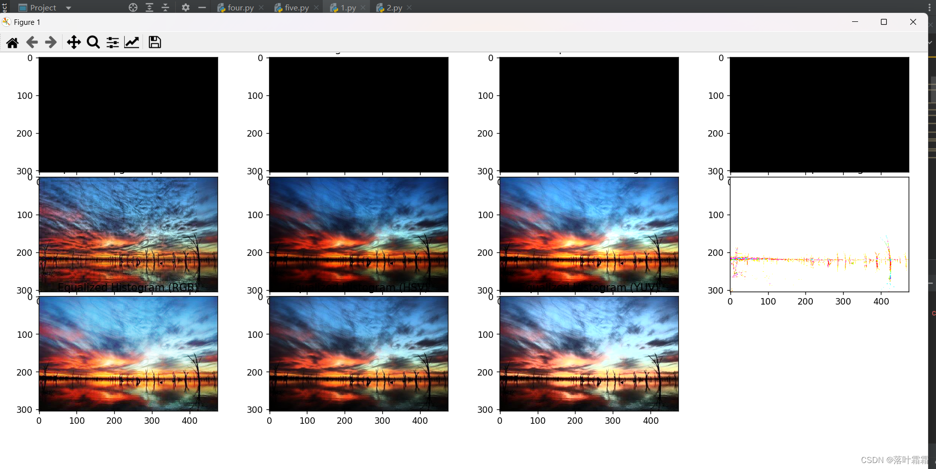
plt.show()输出结果:
小结
有多种方法和技术可用于改善RGB图像的可视效果,但其中许多方法都需要手动调整参数。上述输出展示了使用不同直方图操作生成的亮度校正效果。通过观察,发现HSV调整、指数变换、对比度拉伸和unsharp masking的效果都是令人满意的。
HSV调整:
HSV调整涉及将RGB图像转换为HSV颜色空间并修改强度分量。这种技术似乎在提高图像可视化效果方面取得了令人满意的结果。
指数变换:
指数变换用于根据指数函数调整像素强度。这种方法在提高图像整体亮度和视觉吸引力方面表现出色。
对比度拉伸:
对比度拉伸旨在通过拉伸指定百分位范围内的强度值来增强图像对比度。结果表明,这种技术有效地提高了图像的视觉质量。
Unsharp Masking:
Unsharp masking涉及通过减去模糊版本来创建图像的锐化版本。应用unsharp masking似乎增强了图像的细节和边缘