前置数学知识

1、先验概率和后验概率

先验概率：根据以往经验和分析得到的概率,它往往作为“由因求果”问题中的“因”出现，如$q(x_t|x_{t-1})$

后验概率：指在得到“结果”的信息后重新修正的概率,是“执果寻因”问题中的“因", 如 $p(x_{t-1}|x_t)$

2、条件概率：设$A$、$B$为任意两个事件，若$P(A)>0$,称在已知事件$A$发生的条件下，事件$B$发生的概率为条件概率，记为$P(B|A)$
$$P(B|A)=\frac{P(A,B)}{P(A)}$$

3、乘法公式：
$$P(A,B)=P(B|A)P(A)$$

4、乘法公式一般形式：
$$P(A,B,C)=P(C|B,A)P(B,A)=P(C|B,A)P(B|A)P(A)$$

5、贝叶斯公式：
$$P(A|B)=\frac{P(B|A)P(A)}{P(B)}$$
6、多元贝叶斯公式:
$$P(A|B,C)=\frac{P(A,B,C)}{P(B,C)}=\frac{P(B|A,C)P(A,C)}{P(B,C)}=\frac{P(B|A,C)P(A|C)P(C)}{P(B|C)P(C)}=\frac{P(B|A,C)P(A|C))}{P(B|C)}$$

7、正态分布的叠加性：当有两个独立的正态分布变量$N_1$和$N_2$,它们的均值和方差分别为${\mu }_1$,${\mu }_2$和${\sigma }_1^2$,${\sigma }_2^2$它们的和为$N=a{N}_1+b{N}_2$的均值和方差可以表示如下：
$$\begin{gathered} E(N)=E(a{N}_1+b{N}_2)=a{\mu }_1+b{\mu }_2 \\ Var(N)=Var(a{N}_1+b{N}_2)=a^2{\sigma }_1^2+b^2{\sigma }_2^2 \end{gathered}$$
相减时：
$$\begin{gathered} E(N)=E(a{N}_1-b{N}_2)=a{\mu }_1-b{\mu }_2 \\ Var(N)=Var(a{N}_1-b{N}_2)=a^2{\sigma }_1^2+b^2{\sigma }_2^2 \end{gathered}$$

8、重参数化:从$N(\mu ,{\sigma }^2)$ 采样等价于从$N(0,1)$采样一个$ϵ$,$ϵ\cdot \sigma +\mu$

9、高斯分布的概率密度函数
$$f(x)=\frac{1}{\sqrt{2\pi }\sigma }{e}^{-\frac{(x-\mu {)}^2}{2{\sigma }^2}}$$
10、高斯分布的KL散度公式
$$KL(p|q)=log\frac{{\sigma }_2}{{\sigma }_1}+\frac{{\sigma }^2+({\mu }_1-{\mu }_2{)}^2}{2{\sigma }_2^2}-\frac{1}{2}$$
11、二次函数配方
$$a{x}^2+bx=a(x+\frac{b}{2a}{)}^2+c$$
12、随机变量的期望公式
设$X$是随机变量，$Y=g(X)$,则：
$$E(Y)=E[g(X)]=\{\begin{array}{l}\sum _{k=1}^{\infty }g(x_k)p_k\\ {\int }_{-\infty }^{\infty }g(x)p(x)dx\end{array}$$

13、KL散度公式
$$KL(p(x)|q(x))=E_{x\sim p(x)}[\frac{p(x)}{q(x)}]=\int p(x)\frac{p(x)}{q(x)}dx$$

介绍DDPM

2020年Berkeley提出DDPM（Denoising Diffusion Probabilistic Models），简称扩散模型，是AIGC的核心算法，在生成图像的真实性和多样性方面均超越了GAN，而且训练过程稳定。缺点是计算成本较高，实时推理比较困难，但也有相关技术在时间和空间维度上降低计算量。

扩散模型包括两个过程：前向扩散过程(前向加噪过程)和反向去噪过程。

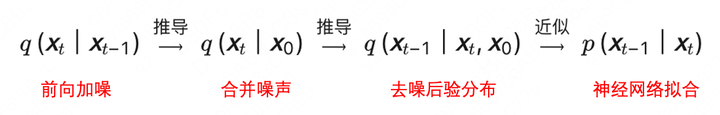
前向过程和反向过程都是马尔可夫链，全过程大约需要1000步，其中反向过程用来生成数据，它的推导过程可以描述成：

前向扩散的过程

前向扩散过程是对原始数据逐渐增加高斯噪声，直至变成标准高斯分布的过程。

从原始数据集采样 $x_0\sim q(x_0)$，按照预定义的noise schedule策略添加随机噪声，得到一系列噪声图像 $x_1,x_2,\dots ,x_T$，用概率表示为：
$$\begin{array}{rl}q(x_{1:T}|x_0)& =\prod _{t=1}^{T}q(x_t|x_{t-1})\\ q(x_t|x_{t-1})& =\mathcal{N}(x_t;\sqrt{{\alpha }_t}{x}_{t-1},{\beta }_{t}I)\end{array}$$
进行重参数化(前置知识数学知识8)，得到
$$\begin{array}{rl}{x}_t& =\sqrt{{\alpha }_t}{x}_{t-1}+\sqrt{{\beta }_t}{ϵ}_t{ϵ}_t\sim \mathcal{N}(0,I)\\ {\alpha }_t& =1-{\beta }_t\end{array}$$

利用上述公式进行迭代推导
$$\begin{array}{rl}{x}_t& =\sqrt{{\alpha }_t}{x}_{t-1}+\sqrt{{\beta }_t}{ϵ}_t\\ & =\sqrt{{\alpha }_t}(\sqrt{{\alpha }_{t-1}}{x}_{t-2}+\sqrt{{\beta }_{t-1}}{ϵ}_{t-1})+\sqrt{{\beta }_t}{ϵ}_t\\ & =\sqrt{({\alpha }_t\dots {\alpha }_1)}{x}_0+\sqrt{({\alpha }_t\dots {\alpha }_2){\beta }_1}{ϵ}_1+\sqrt{({\alpha }_t\dots {\alpha }_3){\beta }_2}{ϵ}_2+\cdots +\sqrt{{\alpha }_t{\beta }_{t-1}}{ϵ}_{t-1}+\sqrt{{\beta }_t}{ϵ}_t\end{array}$$

设：$\overline{{\alpha }_t}={\alpha }_1{\alpha }_2\dots {\alpha }_t$

根据正态分布的叠加性得到

$$\begin{gathered} x_t=\sqrt{\overline{{\alpha }_t}}{x}_0+\sqrt{1-\overline{{\alpha }_t}}ϵϵ\sim \mathcal{N}(0,I) \\ q(x_t|x_0)=\mathcal{N}(x_t;\sqrt{\overline{{\alpha }_t}}{x}_0,\sqrt{1-\overline{{\alpha }_t}}I) \end{gathered}$$
这个公式表示任意步骤$t$的噪声图像$x_t$ ，都可以通过 $x_0$直接加噪得到，后面需要用到。

注：上述前向过程在代码实现时是一步到位的！！！！！

反向去噪过程,神经网络拟合过程

反向去噪过程就是数据生成过程，它首先是从标准高斯分布中采样得到一个噪声样本，再一步步地迭代去噪，最后得到数据分布中的一个样本。

如果知道反向过程的每一步真实的条件分布$q(x_{t-1}|x_t)$，那么从一个随机噪声开始，逐步采样就能生成一个真实的样本。但是真实的条件分布利用贝叶斯公式
$$q(x_{t-1}|x_t)=\frac{q(x_t|x_{t-1})q(x_{t-1})}{q(x_t)}$$
无法直接求解，原因是其中$q(x_{t-1})$ ,$q(x_t)$ 未知，因此无法从$x_t$ 推导到$x_{t-1}$，所以必须通过神经网络**$p_{\theta }(x_{t-1}|x_t)$来近似。为了简化起见，将反向过程也定义为一个马尔卡夫链，且服从高斯分布**，建模如下:

$$\begin{gathered} p_{\theta }(x_{0:T})=p(x_T)\prod _{t=1}^T{p}_{\theta }(x_{t-1}|x_t) \\ {p}_{\theta }(x_{t-1}|x_t)=N(x_{t-1};{\mu }_{\theta }(x_t,t),\sum _{\theta }(x_t,t)) \end{gathered}$$

--------------------下面这段讲解与上面有些跳脱，是为损失函数做铺垫------------------------------

虽然真实条件分布 $q(x_{t-1}|x_t)$无法直接求解，但是加上已知条件 $x_0$的后验分布$q(x_{t-1}|x_{t},x_{0}) $却可以通过贝叶斯公式求解，再结合前向马尔科夫性质可得：
$$q(x_{t-1}|x_t,x_0)=\frac{q(x_t|x_{t-1},x_0)q(x_{t-1}|x_0)}{q(x_t|x_0)}=\frac{q(x_t|x_{t-1})q(x_{t-1}|x_0)}{q(x_t|x_0)}$$
因此可以得到：
$$\begin{array}{rl}q(x_{t-1}|x_0)& =\sqrt{{\bar{\alpha }}_{t-1}}{x}_0+\sqrt{1-{\bar{\alpha }}_{t-1}}ϵ\sim \mathcal{N}(\sqrt{{\bar{\alpha }}_{t-1}}{x}_0,(1-{\bar{\alpha }}_{t-1})I)\\ q(x_t|x_0)& =\sqrt{{\bar{\alpha }}_t}{x}_0+\sqrt{1-{\bar{\alpha }}_t}ϵ\sim \mathcal{N}(\sqrt{{\bar{\alpha }}_t}{x}_0,(1-{\bar{\alpha }}_t)I)\\ q(x_t|x_{t-1})& ={\sqrt{\alpha }}_t{x}_{t-1}+{\beta }_tϵ\sim \mathcal{N}({\sqrt{\alpha }}_t{x}_{t-1},{\beta }_{t}I)\end{array}$$
所以
$$\begin{array}{rl}q(x_{t-1}|x_t,x_0)& \propto exp(-\frac{1}{2}(\frac{(x_t-\sqrt{{\alpha }_t}{x}_{t-1}{)}^2}{{\beta }_t})+\frac{(x_{t-1}-{\sqrt{\bar{\alpha }}}_{t-1}{x}_0{)}^2}{1-{\bar{\alpha }}_{t-1}}-\frac{(x_t-\sqrt{{\bar{\alpha }}_t}{x}_0{)}^2}{1-{\bar{\alpha }}_t})\\ & =exp(-\frac{1}{2}(\frac{{\alpha }_t}{{\beta }_t}+\frac{1}{1-{\bar{\alpha }}_{t-1}})x_{t-1}^2-(\frac{2\sqrt{{\alpha }_t}}{{\beta }_t}{x}_t+\frac{2\sqrt{\overline{{\alpha }_t}}}{1-\overline{{\alpha }_t}}{x}_0)x_{t-1}+C(x_t,x_0))\end{array}$$

通过配方就可以得到
$$\begin{gathered} {\tilde{\beta }}_t=1/(\frac{{\alpha }_t}{{\beta }_t}+\frac{1}{1-{\bar{\alpha }}_{t-1}})=\frac{1-{\bar{\alpha }}_{t-1}}{1-{\bar{\alpha }}_t}{\beta }_t \\ {\tilde{\mu }}_t=(\frac{{\sqrt{\alpha }}_t}{{\beta }_t}{x}_t+\frac{\sqrt{{\bar{\alpha }}_t}}{1-\overline{{\alpha }_t}}{x}_0)/(\frac{{\alpha }_t}{{\beta }_t}+\frac{1}{1-{\bar{\alpha }}_{t-1}})=\frac{\sqrt{{\alpha }_t}(1-{\bar{\alpha }}_{t-1})}{1-\overline{{\alpha }_t}}{x}_t+\frac{\sqrt{{\bar{\alpha }}_{t-1}}{\beta }_t}{1-{\bar{\alpha }}_t}{x}_0 \end{gathered}$$

又因为
$$x_0=\frac{1}{\sqrt{{\bar{\alpha }}_t}}(x_t-\frac{{\beta }_t}{\sqrt{1-{\bar{\alpha }}_t}}ϵ)$$
可以得
$${\tilde{\mu }}_t=\frac{1}{\sqrt{{\alpha }_t}}(x_t-\frac{{\beta }_t}{\sqrt{(1-{\alpha }_t)}}ϵ)$$

----------------------------------------------------------------------------------------------

采样过程（模型训练完后的预测过程）

$$\begin{gathered} {\mu }_{\theta }(x_t,t)=\frac{1}{\sqrt{{\alpha }_t}}(x_t-\frac{{\beta }_t}{\sqrt{(1-{\alpha }_t)}}{ϵ}_{\theta }(x_t,t)) \\ {x}_{t-1}\sim p_{\theta }(x_{t-1}|x_t) \\ {x}_{t-1}=\frac{1}{\sqrt{{\alpha }_t}}(x_t-\frac{{\beta }_t}{\sqrt{(1-{\alpha }_t)}}{ϵ}_{\theta }(x_t,t))+\sqrt{{\tilde{\beta }}_t}zz\sim N(0,I) \end{gathered}$$
这里用z是为了和之前的$ϵ$区别开

损失函数

https://blog.csdn.net/weixin_45453121/article/details/131223653

Code

import torch
import torchvision
import matplotlib.pyplot as plt
import torch.nn.functional as F
from torchvision import transforms
from torch.utils.data import DataLoader
import numpy as np
from torch.optim import Adam
from torch import nn
import math
from torchvision.utils import save_imagedef show_images(data, num_samples=20, cols=4):""" Plots some samples from the dataset """plt.figure(figsize=(15,15))for i, img in enumerate(data):if i == num_samples:breakplt.subplot(int(num_samples/cols) + 1, cols, i + 1)plt.imshow(img[0])def linear_beta_schedule(timesteps, start=0.0001, end=0.02):return torch.linspace(start, end, timesteps)def get_index_from_list(vals, t, x_shape):"""Returns a specific index t of a passed list of values valswhile considering the batch dimension."""batch_size = t.shape[0]out = vals.gather(-1, t.cpu())#print("out:",out)#print("out.shape:",out.shape)return out.reshape(batch_size, *((1,) * (len(x_shape) - 1))).to(t.device)def forward_diffusion_sample(x_0, t, device="cpu"):"""Takes an image and a timestep as input andreturns the noisy version of it"""noise = torch.randn_like(x_0)sqrt_alphas_cumprod_t = get_index_from_list(sqrt_alphas_cumprod, t, x_0.shape)sqrt_one_minus_alphas_cumprod_t = get_index_from_list(sqrt_one_minus_alphas_cumprod, t, x_0.shape)# mean + variancereturn sqrt_alphas_cumprod_t.to(device) * x_0.to(device) \+ sqrt_one_minus_alphas_cumprod_t.to(device) * noise.to(device), noise.to(device)def load_transformed_dataset(IMG_SIZE):data_transforms = [transforms.Resize((IMG_SIZE, IMG_SIZE)),transforms.ToTensor(), # Scales data into [0,1]transforms.Lambda(lambda t: (t * 2) - 1) # Scale between [-1, 1]]data_transform = transforms.Compose(data_transforms)train = torchvision.datasets.MNIST(root="./Data",transform=data_transform,train=True)test = torchvision.datasets.MNIST(root="./Data", transform=data_transform, train=False)return torch.utils.data.ConcatDataset([train, test])def show_tensor_image(image):reverse_transforms = transforms.Compose([transforms.Lambda(lambda t: (t + 1) / 2),transforms.Lambda(lambda t: t.permute(1, 2, 0)), # CHW to HWCtransforms.Lambda(lambda t: t * 255.),transforms.Lambda(lambda t: t.numpy().astype(np.uint8)),transforms.ToPILImage(),])#Take first image of batchif len(image.shape) == 4:image = image[0, :, :, :]plt.imshow(reverse_transforms(image))class Block(nn.Module):def __init__(self, in_ch, out_ch, time_emb_dim, up=False):super().__init__()self.time_mlp =  nn.Linear(time_emb_dim, out_ch)if up:self.conv1 = nn.Conv2d(2*in_ch, out_ch, 3, padding=1)self.transform = nn.ConvTranspose2d(out_ch, out_ch, 4, 2, 1)else:self.conv1 = nn.Conv2d(in_ch, out_ch, 3, padding=1)self.transform = nn.Conv2d(out_ch, out_ch, 4, 2, 1)self.conv2 = nn.Conv2d(out_ch, out_ch, 3, padding=1)self.bnorm1 = nn.BatchNorm2d(out_ch)self.bnorm2 = nn.BatchNorm2d(out_ch)self.relu  = nn.ReLU()def forward(self, x, t):#print("ttt:",t.shape)# First Convh = self.bnorm1(self.relu(self.conv1(x)))# Time embeddingtime_emb = self.relu(self.time_mlp(t))# Extend last 2 dimensionstime_emb = time_emb[(..., ) + (None, ) * 2]# Add time channelh = h + time_emb# Second Convh = self.bnorm2(self.relu(self.conv2(h)))# Down or Upsamplereturn self.transform(h)class SinusoidalPositionEmbeddings(nn.Module):def __init__(self, dim):super().__init__()self.dim = dimdef forward(self, time):device = time.devicehalf_dim = self.dim // 2embeddings = math.log(10000) / (half_dim - 1)embeddings = torch.exp(torch.arange(half_dim, device=device) * -embeddings)embeddings = time[:, None] * embeddings[None, :]embeddings = torch.cat((embeddings.sin(), embeddings.cos()), dim=-1)# TODO: Double check the ordering herereturn embeddingsclass SimpleUnet(nn.Module):"""A simplified variant of the Unet architecture."""def __init__(self):super().__init__()image_channels =1   #灰度图为1，彩色图为3down_channels = (64, 128, 256, 512, 1024)up_channels = (1024, 512, 256, 128, 64)out_dim = 1   #灰度图为1 ，彩色图为3time_emb_dim = 32# Time embeddingself.time_mlp = nn.Sequential(SinusoidalPositionEmbeddings(time_emb_dim),nn.Linear(time_emb_dim, time_emb_dim),nn.ReLU())# Initial projectionself.conv0 = nn.Conv2d(image_channels, down_channels[0], 3, padding=1)# Downsampleself.downs = nn.ModuleList([Block(down_channels[i], down_channels[i+1], \time_emb_dim) \for i in range(len(down_channels)-1)])# Upsampleself.ups = nn.ModuleList([Block(up_channels[i], up_channels[i+1], \time_emb_dim, up=True) \for i in range(len(up_channels)-1)])# Edit: Corrected a bug found by Jakub C (see YouTube comment)self.output = nn.Conv2d(up_channels[-1], out_dim, 1)def forward(self, x, timestep):# Embedd timet = self.time_mlp(timestep)# Initial convx = self.conv0(x)# Unetresidual_inputs = []for down in self.downs:x = down(x, t)residual_inputs.append(x)for up in self.ups:residual_x = residual_inputs.pop()# Add residual x as additional channelsx = torch.cat((x, residual_x), dim=1)x = up(x, t)return self.output(x)def get_loss(model, x_0, t):x_noisy, noise = forward_diffusion_sample(x_0, t, device)noise_pred = model(x_noisy, t)return F.l1_loss(noise, noise_pred)@torch.no_grad()
def sample_timestep(x, t):"""Calls the model to predict the noise in the image and returnsthe denoised image.Applies noise to this image, if we are not in the last step yet."""betas_t = get_index_from_list(betas, t, x.shape)sqrt_one_minus_alphas_cumprod_t = get_index_from_list(sqrt_one_minus_alphas_cumprod, t, x.shape)sqrt_recip_alphas_t = get_index_from_list(sqrt_recip_alphas, t, x.shape)# Call model (current image - noise prediction)model_mean = sqrt_recip_alphas_t * (x - betas_t * model(x, t) / sqrt_one_minus_alphas_cumprod_t)posterior_variance_t = get_index_from_list(posterior_variance, t, x.shape)if t == 0:# As pointed out by Luis Pereira (see YouTube comment)# The t's are offset from the t's in the paperreturn model_meanelse:noise = torch.randn_like(x)return model_mean + torch.sqrt(posterior_variance_t) * noise@torch.no_grad()
def sample_plot_image(IMG_SIZE):# Sample noiseimg_size = IMG_SIZEimg = torch.randn((1, 1, img_size, img_size), device=device)   #生成第T步的图片plt.figure(figsize=(15,15))plt.axis('off')num_images = 10stepsize = int(T/num_images)for i in range(0,T)[::-1]:t = torch.full((1,), i, device=device, dtype=torch.long)#print("t:",t)img = sample_timestep(img, t)# Edit: This is to maintain the natural range of the distributionimg = torch.clamp(img, -1.0, 1.0)if i % stepsize == 0:plt.subplot(1, num_images, int(i/stepsize)+1)plt.title(str(i))show_tensor_image(img.detach().cpu())plt.show()if __name__ =="__main__":# Define beta scheduleT = 300betas = linear_beta_schedule(timesteps=T)# Pre-calculate different terms for closed formalphas = 1. - betasalphas_cumprod = torch.cumprod(alphas, axis=0)# print(alphas_cumprod.shape)alphas_cumprod_prev = F.pad(alphas_cumprod[:-1], (1, 0), value=1.0)# print(alphas_cumprod_prev)# print(alphas_cumprod_prev.shape)sqrt_recip_alphas = torch.sqrt(1.0 / alphas)sqrt_alphas_cumprod = torch.sqrt(alphas_cumprod)sqrt_one_minus_alphas_cumprod = torch.sqrt(1. - alphas_cumprod)posterior_variance = betas * (1. - alphas_cumprod_prev) / (1. - alphas_cumprod)# print(posterior_variance.shape)IMG_SIZE = 32BATCH_SIZE = 16data = load_transformed_dataset(IMG_SIZE)dataloader = DataLoader(data, batch_size=BATCH_SIZE, shuffle=True, drop_last=True)model = SimpleUnet()print("Num params: ", sum(p.numel() for p in model.parameters()))device = "cuda" if torch.cuda.is_available() else "cpu"model.to(device)optimizer = Adam(model.parameters(), lr=0.001)epochs = 1 # Try more!for epoch in range(epochs):for step, batch in enumerate(dataloader):  #由于batch 是包含标签的所以取batch[0]#print(batch[0].shape)optimizer.zero_grad()t = torch.randint(0, T, (BATCH_SIZE,), device=device).long()loss = get_loss(model, batch[0], t)loss.backward()optimizer.step()if epoch % 1 == 0 and step %5== 0:print(f"Epoch {epoch} | step {step:03d} Loss: {loss.item()} ")sample_plot_image(IMG_SIZE)

参考文献

https://zhuanlan.zhihu.com/p/630354327](https://zhuanlan.zhihu.com/p/630354327)

https://blog.csdn.net/weixin_45453121/article/details/131223653

https://www.cnblogs.com/risejl/p/17448442.html

https://zhuanlan.zhihu.com/p/569994589?utm_id=0