BERT模型的网络结构解析运行案例分析

整体结构

第一部分：嵌入层
第二部分：编码层
第三部分：输出层

对于一个m分类任务，输入n个词作为一次数据，单个批次输入t个数据，在BERT模型的不同部分，数据的形状信息如下：
注1：m = num_classes，n = sequence_length，t = batch_size，根据数据的形状和维度信息，可以加深对模型的理解
注2：一个具体的例子，输入n个单词形成一句话，判断这句话是否自然（二分类，语句自然输出1，否则输出0，此时m=2），为了加速计算，单个批次输入t个句子进行并行处理。

嵌入层（Embedding Layer）：
- 输入数据形状：(batch_size, sequence_length)
- 输出数据形状：(batch_size, sequence_length, embedding_dim)
- 其中，embedding_dim 是词嵌入的维度，通常是固定的，例如在BERT中，embedding_dim 为768。
编码层（Encoder Layers）：
- 输入数据形状：(batch_size, sequence_length, embedding_dim)
- 输出数据形状：(batch_size, sequence_length, hidden_size)
- 其中，hidden_size 是编码层输出的隐藏状态的维度，通常也是固定的，例如在BERT中，hidden_size 为768。
输出层（Output Layer）：
- 输入数据形状：(batch_size, sequence_length, hidden_size)
- 输出数据形状：(batch_size, num_classes)
- 其中，num_classes 是分类任务的类别数，通常是固定的，表示输出层的神经元数量。

为了方便表示，后续均以单次数据的处理为准，对于批次数据，数据形状前面加一个维度即可。比如对于单次输入，即为(sequence_length,)；对于批次输入，即为(batch_size, sequence_length)。

第一部分：嵌入层

BERT模型的嵌入层结构包括以下几个部分：

Token Embeddings：Token Embeddings 是将输入的词汇（token）映射为词向量（word embeddings）的过程。对于BERT模型而言，通常使用的是WordPiece或者Byte Pair Encoding（BPE）等子词级别的编码方式。每个词汇被映射为一个固定长度的词向量，例如在BERT-base模型中，词向量的维度为768。
Positional Embeddings：Positional Embeddings 是用于表示输入序列中每个词汇的位置信息的嵌入向量。由于BERT模型是基于Transformer结构的，它不具备循环神经网络（RNN）等具有顺序感知性的结构，因此需要通过Positional Embeddings来引入位置信息。通常，位置编码采用的是一组特殊设计的固定向量，以表示每个位置的绝对位置信息和相对位置信息。
Segment Embeddings：Segment Embeddings 是用于区分不同句子或文本片段的嵌入向量。在BERT模型中，输入文本通常由两个句子组成，分别表示为句子A和句子B。Segment Embeddings用于区分这两个句子，以便模型能够理解和处理它们之间的关系。在BERT模型中，通常将句子A的Segment Embeddings设置为0，句子B的Segment Embeddings设置为1。

这些嵌入向量会被按元素加和，形成最终的输入表示，作为编码层（Encoder Layers）的输入。在BERT模型中，这些嵌入向量的长度会与输入序列的长度相同，但是每个向量的维度（通常是768）是由模型的超参数决定的。

对于单个数据，输入n个词，涉及的数据形状可以描述如下：

词嵌入（Token Embeddings）：
- 数据形状：(n, embedding_dim)
- 这是将每个token映射为词向量后得到的数据形状，其中embedding_dim是词向量的维度，例如在BERT中通常是768。
位置嵌入（Positional Embeddings）：
- 数据形状：(n, embedding_dim)
- 这是表示每个token在序列中位置信息的嵌入向量，与词嵌入具有相同的维度（一般为768），每个位置的嵌入向量都不同。
段落嵌入（Segment Embeddings）：
- 数据形状：(n, embedding_dim)
- 这是表示每个token所属句子（段落）的嵌入向量，与词嵌入具有相同的维度（一般为768），通常在BERT模型中，第一个句子的段落嵌入为0，第二个句子的段落嵌入为1。

对于前面介绍的具体例子：

输入n个单词形成一句话，判断这句话是否自然

打印模型的结构信息可以看到如下内容：

(word_embeddings): Embedding(30522, 768)
(position_embeddings): Embedding(512, 768)
(token_type_embeddings): Embedding(2, 768)

对于这个模型，有30522个单词，每个单词对应一行长度为768的向量；输入限制长度512个单词，位置有512个向量，每个位置对应一行长度为768的向量；由于模型最多只能往里面输入两句话，即段落嵌入对于单个词不是0就是1，因此有2行代表两句话，每句话对应一行长度为768的向量。

比如输入文本what is your name，转化为词元序列可能为[84, 79, 105, 97]，对应word_embeddings的第84行，79行，105行，97行的向量w0, w1, w2, w3，那么经过词嵌入Token Embeddings后变为[w0, w1, w2, w3]，形状为(4, 768)，记该矩阵为W_word。

对于位置，即为[0, 1, 2, 3]，对应Positional Embeddings的第0行，第1行，第2行，第3行，同上得到位置嵌入后结果为[p0, p1, p2, p3]，形状为(4, 768)，记该矩阵为P_word。

对于段落，由于上述例子只使用了一句话，可以是[0, 0, 0, 0]，同理段落嵌入后为[s0, s0, s0, s0]，形状为(4, 768)，记该矩阵为S_word。假如是两句话what is your name my name is x，那么段落序列可能就是[0, 0, 0, 0, 1, 1, 1, 1]

最后的输入需要汇总三种信息，直接相加：input = W_word + P_word + S_word，形状最后变为(4, 768)。

实际模型里面，做完这些还需做额外处理，打印模型结构信息如下：

(embeddings): BertEmbeddings((word_embeddings): Embedding(30522, 768)(position_embeddings): Embedding(512, 768)(token_type_embeddings): Embedding(2, 768)(LayerNorm): LayerNorm((768,))(dropout): Dropout(p=0.1))

额外处理就是两层网络来完成：LayerNorm做归一化处理，提高计算稳定性；dropout按照概率p=0.1随机让一部分输出暂停，缓解过拟合现象。这两层都是神经网络模型基础操作，在此不深入讨论。

第二部分：编码层

BERT（Bidirectional Encoder Representations from Transformers）模型的编码层结构主要基于Transformer架构。在BERT中，编码层由多个Transformer块组成，每个Transformer块都包含了多个自注意力层（Self-Attention Layer）和前馈神经网络层（Feedforward Neural Network Layer）。

具体来说，BERT的编码层结构如下：

Transformer块（Transformer Block）：BERT模型通常由多个Transformer块组成。每个Transformer块都包含了多个子层，包括多头自注意力层和前馈神经网络层。在BERT-base模型中，通常有12个Transformer块，而在BERT-large模型中，通常有24个Transformer块。
多头自注意力层（Multi-Head Self-Attention Layer）：自注意力层用于计算输入序列中每个token的表示，其中每个token都会考虑到其他token的信息。在BERT中，自注意力层被分为多个头（head），每个头都学习到了不同的注意力权重，然后将多个头的输出进行拼接和线性变换以得到最终的自注意力表示。
前馈神经网络层（Feedforward Neural Network Layer）：前馈神经网络层用于在每个位置上对输入进行非线性变换。在BERT中，前馈神经网络层通常是一个全连接层，其输入是自注意力层的输出，输出是一个具有固定维度的向量。

在BERT模型中，编码层的作用是对输入序列进行多层次的特征提取和表示学习，以便为下游任务提供丰富的语义信息。通过堆叠多个Transformer块，BERT模型能够捕捉输入序列中的复杂关系和长程依赖关系，从而实现了在大规模文本数据上的预训练和迁移学习。

实际模型里面，我们打印编码层的网络结构信息看看（看起来内容还挺多，我们后面慢慢拆解来看）：

(encoder): BertEncoder((layer): ModuleList((0-11): 12 x BertLayer((attention): BertAttention((self): BertSelfAttention((query): Linear(in_features=768, out_features=768, bias=True)(key): Linear(in_features=768, out_features=768, bias=True)(value): Linear(in_features=768, out_features=768, bias=True)(dropout): Dropout(p=0.1, inplace=False))(output): BertSelfOutput((dense): Linear(in_features=768, out_features=768, bias=True)(LayerNorm): LayerNorm((768,), eps=1e-12, elementwise_affine=True)(dropout): Dropout(p=0.1, inplace=False)))(intermediate): BertIntermediate((dense): Linear(in_features=768, out_features=3072, bias=True)(intermediate_act_fn): GELUActivation())(output): BertOutput((dense): Linear(in_features=3072, out_features=768, bias=True)(LayerNorm): LayerNorm((768,), eps=1e-12, elementwise_affine=True)(dropout): Dropout(p=0.1, inplace=False)))))

总的来说，编码层由12个编码器组成，每个编码器都有相同的结构，因此我们只需要解析单个编码器结构即可，单个编码器得到网络结构信息如下（嗯，内容虽然有所缩减，但依然较多）：

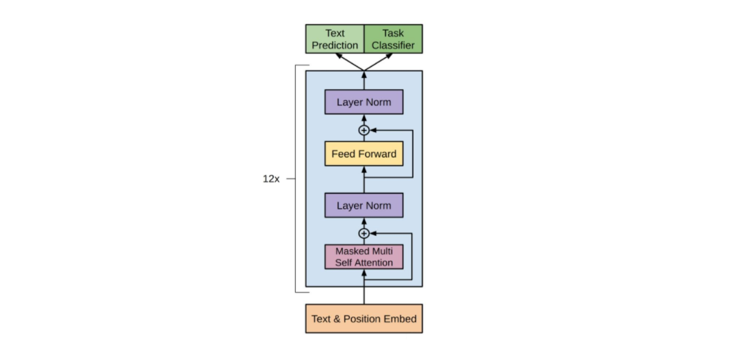
            (attention): BertAttention((self): BertSelfAttention((query): Linear(in_features=768, out_features=768, bias=True)(key): Linear(in_features=768, out_features=768, bias=True)(value): Linear(in_features=768, out_features=768, bias=True)(dropout): Dropout(p=0.1, inplace=False))(output): BertSelfOutput((dense): Linear(in_features=768, out_features=768, bias=True)(LayerNorm): LayerNorm((768,), eps=1e-12, elementwise_affine=True)(dropout): Dropout(p=0.1, inplace=False)))(intermediate): BertIntermediate((dense): Linear(in_features=768, out_features=3072, bias=True)(intermediate_act_fn): GELUActivation())(output): BertOutput((dense): Linear(in_features=3072, out_features=768, bias=True)(LayerNorm): LayerNorm((768,), eps=1e-12, elementwise_affine=True)(dropout): Dropout(p=0.1, inplace=False))

每个编码器包含两个子层，包括多头自注意力层和前馈神经网络层。其实，就是这么一个玩意儿：

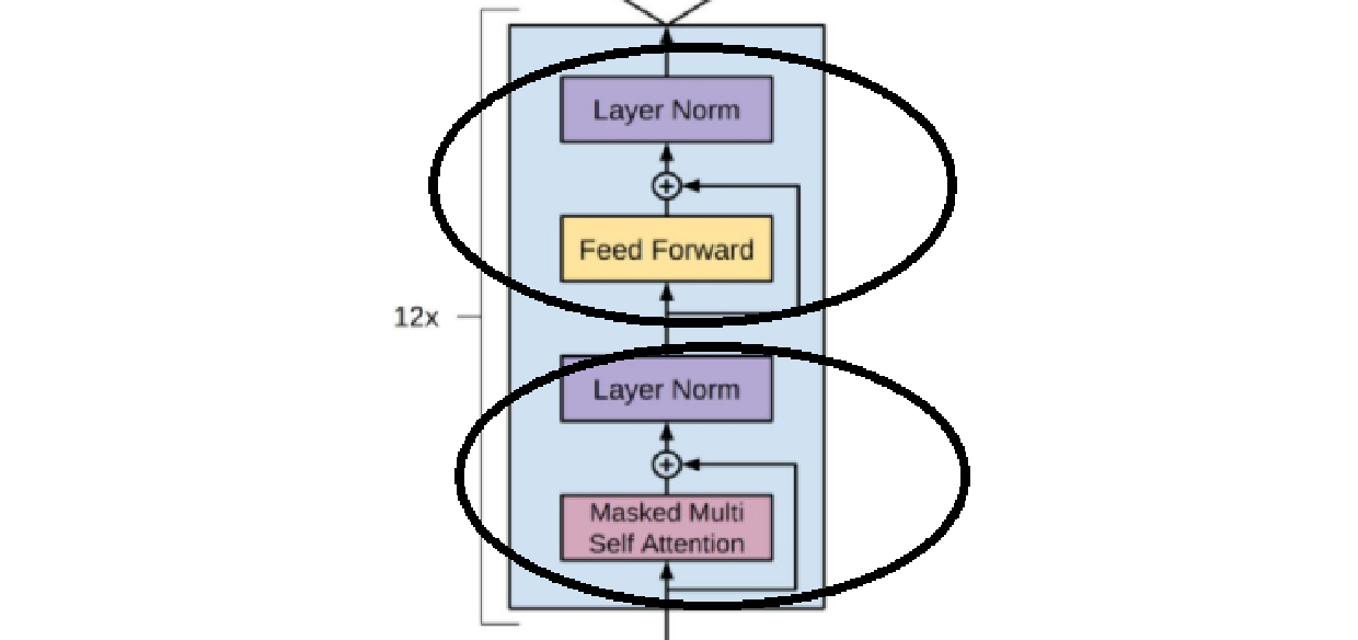
上面的是前馈神经网络层，下面的是多头自注意力层。多头自注意力层的模型结构信息如下，结合transformer的那一坨东西很容易就能看懂：

(attention): BertAttention((self): BertSelfAttention((query): Linear(in_features=768, out_features=768, bias=True)(key): Linear(in_features=768, out_features=768, bias=True)(value): Linear(in_features=768, out_features=768, bias=True)(dropout): Dropout(p=0.1, inplace=False))(output): BertSelfOutput((dense): Linear(in_features=768, out_features=768, bias=True)(LayerNorm): LayerNorm((768,), eps=1e-12, elementwise_affine=True)(dropout): Dropout(p=0.1, inplace=False)))

简单来说，就是一个QKV运算+残差归一化。同理，结合transformer也很容易看懂如下的前馈神经网络层：

(intermediate): BertIntermediate((dense): Linear(in_features=768, out_features=3072, bias=True)(intermediate_act_fn): GELUActivation())(output): BertOutput((dense): Linear(in_features=3072, out_features=768, bias=True)(LayerNorm): LayerNorm((768,), eps=1e-12, elementwise_affine=True)(dropout): Dropout(p=0.1, inplace=False))

搞这么一层无非就是为了函数的非线性特征，那个非线性激活函数GELUActivation()才是重点。

现在来大概梳理一下，编码层由12个编码器“串联”，单个编码器输入输入数据的形状都没有变，对于单次数据，输入输出形状均为：(max_seq_length, embedding_dim)。而在编码器内部的处理中，会存在更大的形状进行特征提取和处理。

第三部分：输出层

依然是针对前面语句是否自然的二分类问题，先看看输出层模型结构有什么：

 (pooler): BertPooler((dense): Linear(in_features=768, out_features=768, bias=True)(activation): Tanh())
(dropout): Dropout(p=0.1, inplace=False)
(classifier): Linear(in_features=768, out_features=2, bias=True)

可以看到，大概就是三个主要的东西：池化层pooler，dropout层（防止过拟合），n分类层（此处为二分类）。n分类层大概用softmax的操作就可以实现，很普通，现在主要看看这个令人十分疑惑的池化层pooler。

BertPooler是BERT模型中的一个组件，用于汇总整个输入序列的表示并生成一个固定长度的向量。在BERT模型中，BertPooler位于最后一层的输出之后，负责将整个序列的表示转化为一个用于下游任务的固定长度的向量。

具体来说，BertPooler使用了最大池化（Max Pooling）操作，它将最后一层的所有词的隐藏状态向量中的最后一个词的隐藏状态向量提取出来，并通过一个全连接层（通常是一个线性变换）和激活函数（通常是tanh函数）来将其转化为一个固定长度的向量。这个向量可以看作是整个输入序列的表示，用于下游任务的进一步处理，如分类或回归。

总之，BertPooler是BERT模型中用于生成整个输入序列的表示的组件，它通过最大池化操作和线性变换将输入序列转化为一个固定长度的向量，以供后续任务使用。

这么说依然会让人倍感疑惑，来一个简单的例子就好了：

好的，让我用一个简单的例子来说明BertPooler是如何操作的。

假设我们有一个输入序列，包含三个词：[“apple”, “banana”, “orange”]。每个词都被BERT编码器转换为一个长度为768的隐藏状态向量。这个序列经过BERT模型后，得到的编码器输出为：

[[0.1, 0.2, ..., 0.3],  # 长度为768的向量，表示"apple"的隐藏状态[0.2, 0.3, ..., 0.4],  # 长度为768的向量，表示"banana"的隐藏状态[0.3, 0.4, ..., 0.5]   # 长度为768的向量，表示"orange"的隐藏状态
]

在BertPooler中，我们使用最大池化操作，即取最后一个词（“orange”）的隐藏状态向量作为整个序列的表示。所以，我们取得到的向量是 [0.3, 0.4, ..., 0.5]。

然后，我们将这个向量输入到一个全连接层（通常是一个线性变换），并通过激活函数（通常是tanh函数）来将其转化为一个固定长度的向量。假设全连接层的权重是随机初始化的，经过线性变换和tanh函数后，得到的固定长度向量可能是：

[0.7, -0.1, 0.5, ..., -0.3]  # 长度为固定长度的向量，作为整个输入序列的表示

这个向量就是BertPooler生成的，它捕获了整个输入序列的语义信息，并用于后续的下游任务，比如分类或回归。

或许这么说还是存在不明不白的地方，那么思考一下：对于768维，池化的过程是针对每一个分量取最大值吗？

对于BertPooler中的最大池化过程，它是针对每个隐藏状态向量的每个分量分别进行比较，然后取每个分量的最大值。具体来说，如果每个隐藏状态向量的长度是768维，则最大池化会从这768个维度中分别选取最大值，形成一个新的768维向量。

举个例子，假设有两个隐藏状态向量：

向量1：[0.1, 0.5, 0.3, …, 0.7]

向量2：[0.4, 0.2, 0.8, …, 0.6]

在最大池化过程中，将分别从这两个向量的每个维度中选取最大值：

[max(0.1, 0.4), max(0.5, 0.2), max(0.3, 0.8), …, max(0.7, 0.6)]

得到的新向量就是每个维度上的最大值所构成的向量。这个过程确保了最大池化能够捕获每个隐藏状态向量中的最显著特征，以生成整个序列的表示。

代码展示

说实话，很多论文和书籍的transformer代码复现是真的臭，能跑通真得天天烧高香。本人侥幸跑通了一份BERT的代码（不保证其他人能跑通），针对的问题就是上面的语句是否自然的二分类问题，代码就附给有缘的冤大头了：
数据在这里：https://github.com/Denis2054/Transformers-for-NLP-2nd-Edition/tree/main/Chapter03

#@title Importing the modules
import torch
import torch.nn as nn
from torch.utils.data import TensorDataset, DataLoader, RandomSampler, SequentialSampler
from keras.preprocessing.sequence import pad_sequences
from sklearn.model_selection import train_test_split
from transformers import BertTokenizer, BertConfig
from transformers import AdamW, BertForSequenceClassification, get_linear_schedule_with_warmup
from tqdm import tqdm, trange
import pandas as pd
import numpy as np
import matplotlib.pyplot as plt#March 2023 update:
#% matplotlib inline
device = torch.device("cuda" if torch.cuda.is_available() else "cpu")
print(f"device = {device}")
df = pd.read_csv("in_domain_train.tsv", delimiter='\t', header=None,names=['sentence_source', 'label', 'label_notes', 'sentence'])
print(f"df.shape = {df.shape}")
print(f"df.sample10 = {df.sample(10)}")
#@ Creating sentence, label lists and adding Bert tokens
sentences = df.sentence.values# Adding CLS and SEP tokens at the beginning and end of each sentence for BERT
sentences = ["[CLS] " + sentence + " [SEP]" for sentence in sentences]
labels = df.label.values
#@title Activating the BERT Tokenizer
tokenizer = BertTokenizer.from_pretrained('bert-base-uncased', do_lower_case=True)
tokenized_texts = [tokenizer.tokenize(sent) for sent in sentences]
print("Tokenize the first sentence:")
print(tokenized_texts[0])
#@title Processing the data
# Set the maximum sequence length. The longest sequence in our training set is 47, but we'll leave room on the end anyway.
# In the original paper, the authors used a length of 512.
MAX_LEN = 128# Use the BERT tokenizer to convert the tokens to their index numbers in the BERT vocabulary
input_ids = [tokenizer.convert_tokens_to_ids(x) for x in tokenized_texts]# Pad our input tokens
input_ids = pad_sequences(input_ids, maxlen=MAX_LEN, dtype="long", truncating="post", padding="post")
print(f"input_ids.shape = {input_ids.shape}")
print(f"input_ids[0] = {input_ids[0]}")
#@title Create attention masks
attention_masks = []# Create a mask of 1s for each token followed by 0s for padding
for seq in input_ids:seq_mask = [float(i > 0) for i in seq]attention_masks.append(seq_mask)
print(f"attention_masks[0] = {attention_masks[0]}")
#@title Splitting data into train and validation sets
# Use train_test_split to split our data into train and validation sets for trainingtrain_inputs, validation_inputs, train_labels, validation_labels = train_test_split(input_ids, labels,random_state=2018, test_size=0.1)
train_masks, validation_masks, _, _ = train_test_split(attention_masks, input_ids,random_state=2018, test_size=0.1)
#@title Converting all the data into torch tensors
# Torch tensors are the required datatype for our modeltrain_inputs = torch.tensor(train_inputs)
validation_inputs = torch.tensor(validation_inputs)
train_labels = torch.tensor(train_labels)
validation_labels = torch.tensor(validation_labels)
train_masks = torch.tensor(train_masks)
validation_masks = torch.tensor(validation_masks)#@title Selecting a Batch Size and Creating and Iterator
# Select a batch size for training. For fine-tuning BERT on a specific task, the authors recommend a batch size of 16 or 32
batch_size = 32# Create an iterator of our data with torch DataLoader. This helps save on memory during training because, unlike a for loop,
# with an iterator the entire dataset does not need to be loaded into memorytrain_data = TensorDataset(train_inputs, train_masks, train_labels)
train_sampler = RandomSampler(train_data)
train_dataloader = DataLoader(train_data, sampler=train_sampler, batch_size=batch_size)validation_data = TensorDataset(validation_inputs, validation_masks, validation_labels)
validation_sampler = SequentialSampler(validation_data)
validation_dataloader = DataLoader(validation_data, sampler=validation_sampler, batch_size=batch_size)# @title Bert Model Configuration
# Initializing a BERT bert-base-uncased style configuration
# @title Transformer Installation
try:import transformers
except:print("Installing transformers")from transformers import BertModel, BertConfigconfiguration = BertConfig()# Initializing a model from the bert-base-uncased style configuration
model = BertModel(configuration)# Accessing the model configuration
configuration = model.config
print(configuration)#@title Loading the Hugging Face Bert Uncased Base Model
model = BertForSequenceClassification.from_pretrained("bert-base-uncased", num_labels=2)
model = nn.DataParallel(model)
model.to(device)# 打印网络结构信息
print("----------------")
print("模型的网络结构信息：")
print(model)
print("----------------")
LP = list(model.parameters())
lp = len(LP)
print(f"matrix num = {lp}")
nps = 0
for p in range(0, lp):  #number of tensorsPL2 = Truetry:L2 = len(LP[p][0])  #check if 2Dexcept:L2 = 1  #not 2D but 1DPL2 = FalseL1 = len(LP[p])L3 = L1 * L2nps += L3  # number of parameters per tensorif PL2 == True:print(p, L1, L2, L3)  # displaying the sizes of the parametersif PL2 == False:print(p, L1, L3)  # displaying the sizes of the parametersprint(nps)  # total number of parameters##@title Optimizer Grouped Parameters
# This code is taken from:
# https://github.com/huggingface/transformers/blob/5bfcd0485ece086ebcbed2d008813037968a9e58/examples/run_glue.py#L102# Don't apply weight decay to any parameters whose names include these tokens.
# (Here, the BERT doesn't have `gamma` or `beta` parameters, only `bias` terms)
param_optimizer = list(model.named_parameters())
no_decay = ['bias', 'LayerNorm.weight']
# Separate the `weight` parameters from the `bias` parameters.
# - For the `weight` parameters, this specifies a 'weight_decay_rate' of 0.01.
# - For the `bias` parameters, the 'weight_decay_rate' is 0.0.
optimizer_grouped_parameters = [# Filter for all parameters which *don't* include 'bias', 'gamma', 'beta'.{'params': [p for n, p in param_optimizer if not any(nd in n for nd in no_decay)],'weight_decay_rate': 0.1},# Filter for parameters which *do* include those.{'params': [p for n, p in param_optimizer if any(nd in n for nd in no_decay)],'weight_decay_rate': 0.0}
]
# Note - `optimizer_grouped_parameters` only includes the parameter values, not
# the names.#@title The Hyperparameters for the Training Loop
# optimizer = BertAdam(optimizer_grouped_parameters,
#                      lr=2e-5,
#                      warmup=.1)# Number of training epochs (authors recommend between 2 and 4)
epochs = 4optimizer = AdamW(optimizer_grouped_parameters,lr=2e-5,  # args.learning_rate - default is 5e-5, our notebook had 2e-5eps=1e-8  # args.adam_epsilon  - default is 1e-8.)
# Total number of training steps is number of batches * number of epochs.
# `train_dataloader` contains batched data so `len(train_dataloader)` gives
# us the number of batches.
total_steps = len(train_dataloader) * epochs# Create the learning rate scheduler.
scheduler = get_linear_schedule_with_warmup(optimizer,num_warmup_steps=0,  # Default value in run_glue.pynum_training_steps=total_steps)#Creating the Accuracy Measurement Function
# Function to calculate the accuracy of our predictions vs labels
def flat_accuracy(preds, labels):pred_flat = np.argmax(preds, axis=1).flatten()labels_flat = labels.flatten()return np.sum(pred_flat == labels_flat) / len(labels_flat)print("everything is fine")# @title The Training Loop
t = []# Store our loss and accuracy for plotting
train_loss_set = []# trange is a tqdm wrapper around the normal python range
for _ in trange(epochs, desc="Epoch"):# Training# Set our model to training mode (as opposed to evaluation mode)model.train()# Tracking variablestr_loss = 0nb_tr_examples, nb_tr_steps = 0, 0# Train the data for one epochfor step, batch in enumerate(train_dataloader):# Add batch to GPUbatch = tuple(t.to(device) for t in batch)# Unpack the inputs from our dataloaderb_input_ids, b_input_mask, b_labels = batch# Clear out the gradients (by default they accumulate)optimizer.zero_grad()# Forward passoutputs = model(b_input_ids, token_type_ids=None, attention_mask=b_input_mask, labels=b_labels)loss = outputs['loss']train_loss_set.append(loss.item())# Backward passloss.backward()# Update parameters and take a step using the computed gradientoptimizer.step()# Update the learning rate.scheduler.step()# Update tracking variablestr_loss += loss.item()nb_tr_examples += b_input_ids.size(0)nb_tr_steps += 1print("Train loss: {}".format(tr_loss / nb_tr_steps))# Validation# Put model in evaluation mode to evaluate loss on the validation setmodel.eval()# Tracking variableseval_loss, eval_accuracy = 0, 0nb_eval_steps, nb_eval_examples = 0, 0# Evaluate data for one epochfor batch in validation_dataloader:# Add batch to GPUbatch = tuple(t.to(device) for t in batch)# Unpack the inputs from our dataloaderb_input_ids, b_input_mask, b_labels = batch# Telling the model not to compute or store gradients, saving memory and speeding up validationwith torch.no_grad():# Forward pass, calculate logit predictionslogits = model(b_input_ids, token_type_ids=None, attention_mask=b_input_mask)# Move logits and labels to CPUlogits = logits['logits'].detach().cpu().numpy()label_ids = b_labels.to('cpu').numpy()tmp_eval_accuracy = flat_accuracy(logits, label_ids)eval_accuracy += tmp_eval_accuracynb_eval_steps += 1print("Validation Accuracy: {}".format(eval_accuracy / nb_eval_steps))#@title Training Evaluation
plt.figure(figsize=(15, 8))
plt.title("Training loss")
plt.xlabel("Batch")
plt.ylabel("Loss")
plt.plot(train_loss_set)
plt.show()# @title Predicting and Evaluating Using the Holdout Dataset
df = pd.read_csv("out_of_domain_dev.tsv", delimiter='\t', header=None,names=['sentence_source', 'label', 'label_notes', 'sentence'])# Create sentence and label lists
sentences = df.sentence.values# We need to add special tokens at the beginning and end of each sentence for BERT to work properly
sentences = ["[CLS] " + sentence + " [SEP]" for sentence in sentences]
labels = df.label.valuestokenized_texts = [tokenizer.tokenize(sent) for sent in sentences]MAX_LEN = 128# Use the BERT tokenizer to convert the tokens to their index numbers in the BERT vocabulary
input_ids = [tokenizer.convert_tokens_to_ids(x) for x in tokenized_texts]
# Pad our input tokens
input_ids = pad_sequences(input_ids, maxlen=MAX_LEN, dtype="long", truncating="post", padding="post")
# Create attention masks
attention_masks = []# Create a mask of 1s for each token followed by 0s for padding
for seq in input_ids:seq_mask = [float(i > 0) for i in seq]attention_masks.append(seq_mask)prediction_inputs = torch.tensor(input_ids)
prediction_masks = torch.tensor(attention_masks)
prediction_labels = torch.tensor(labels)batch_size = 32prediction_data = TensorDataset(prediction_inputs, prediction_masks, prediction_labels)
prediction_sampler = SequentialSampler(prediction_data)
prediction_dataloader = DataLoader(prediction_data, sampler=prediction_sampler, batch_size=batch_size)# Prediction on test set# Put model in evaluation mode
model.eval()# Tracking variables
predictions, true_labels = [], []# Predict
for batch in prediction_dataloader:# Add batch to GPUbatch = tuple(t.to(device) for t in batch)# Unpack the inputs from our dataloaderb_input_ids, b_input_mask, b_labels = batch# Telling the model not to compute or store gradients, saving memory and speeding up predictionwith torch.no_grad():# Forward pass, calculate logit predictionslogits = model(b_input_ids, token_type_ids=None, attention_mask=b_input_mask)# Move logits and labels to CPUlogits = logits['logits'].detach().cpu().numpy()label_ids = b_labels.to('cpu').numpy()# Store predictions and true labelspredictions.append(logits)true_labels.append(label_ids)#@title Evaluating Using Matthew's Correlation Coefficient
# Import and evaluate each test batch using Matthew's correlation coefficient
from sklearn.metrics import matthews_corrcoef
matthews_set = []for i in range(len(true_labels)):matthews = matthews_corrcoef(true_labels[i],np.argmax(predictions[i], axis=1).flatten())matthews_set.append(matthews)#@title Score of Individual Batches
print(f"Matthews Correlation: {matthews_set}")flat_predictions = [item for sublist in predictions for item in sublist]
flat_predictions = np.argmax(flat_predictions, axis=1).flatten()
flat_true_labels = [item for sublist in true_labels for item in sublist]
matthews_all = matthews_corrcoef(flat_true_labels, flat_predictions)
print(f"Matthews Correlation All: {matthews_all}")

输出：

2024-05-06 10:16:24.198115: I tensorflow/core/util/port.cc:113] oneDNN custom operations are on. You may see slightly different numerical results due to floating-point round-off errors from different computation orders. To turn them off, set the environment variable `TF_ENABLE_ONEDNN_OPTS=0`.
2024-05-06 10:16:24.584165: I tensorflow/core/util/port.cc:113] oneDNN custom operations are on. You may see slightly different numerical results due to floating-point round-off errors from different computation orders. To turn them off, set the environment variable `TF_ENABLE_ONEDNN_OPTS=0`.
device = cuda
df.shape = (8551, 4)
df.sample10 =      sentence_source  ...                                           sentence
5846            c_13  ...             i asked for him to eat the asparagus .
3865            ks08  ...                frank threw himself into the sofa .
4334            ks08  ...  gregory appears to have wanted to be loyal to ...
5423            b_73  ...          we made enough pudding to last for days .
4338            ks08  ...      he coaxed his brother to give him the candy .
5680            c_13  ...           the canadian bought himself a barbecue .
2362            l-93  ...                   the horse kicked penny 's shin .
5841            c_13  ...                   i think that he eats asparagus .
1284            r-67  ...        tony has a fiat to yearn for a tall nurse .
3021            l-93  ...                       i was hunting in the woods .[10 rows x 4 columns]
D:\Program\Python312\Lib\site-packages\huggingface_hub\file_download.py:1132: FutureWarning: `resume_download` is deprecated and will be removed in version 1.0.0. Downloads always resume when possible. If you want to force a new download, use `force_download=True`.warnings.warn(
Tokenize the first sentence:
['[CLS]', 'our', 'friends', 'wo', 'n', "'", 't', 'buy', 'this', 'analysis', ',', 'let', 'alone', 'the', 'next', 'one', 'we', 'propose', '.', '[SEP]']
input_ids.shape = (8551, 128)
input_ids[0] = [  101  2256  2814 24185  1050  1005  1056  4965  2023  4106  1010  22922894  1996  2279  2028  2057 16599  1012   102     0     0     0     00     0     0     0     0     0     0     0     0     0     0     00     0     0     0     0     0     0     0     0     0     0     00     0     0     0     0     0     0     0     0     0     0     00     0     0     0     0     0     0     0     0     0     0     00     0     0     0     0     0     0     0     0     0     0     00     0     0     0     0     0     0     0     0     0     0     00     0     0     0     0     0     0     0     0     0     0     00     0     0     0     0     0     0     0     0     0     0     00     0     0     0     0     0     0     0]
attention_masks[0] = [1.0, 1.0, 1.0, 1.0, 1.0, 1.0, 1.0, 1.0, 1.0, 1.0, 1.0, 1.0, 1.0, 1.0, 1.0, 1.0, 1.0, 1.0, 1.0, 1.0, 0.0, 0.0, 0.0, 0.0, 0.0, 0.0, 0.0, 0.0, 0.0, 0.0, 0.0, 0.0, 0.0, 0.0, 0.0, 0.0, 0.0, 0.0, 0.0, 0.0, 0.0, 0.0, 0.0, 0.0, 0.0, 0.0, 0.0, 0.0, 0.0, 0.0, 0.0, 0.0, 0.0, 0.0, 0.0, 0.0, 0.0, 0.0, 0.0, 0.0, 0.0, 0.0, 0.0, 0.0, 0.0, 0.0, 0.0, 0.0, 0.0, 0.0, 0.0, 0.0, 0.0, 0.0, 0.0, 0.0, 0.0, 0.0, 0.0, 0.0, 0.0, 0.0, 0.0, 0.0, 0.0, 0.0, 0.0, 0.0, 0.0, 0.0, 0.0, 0.0, 0.0, 0.0, 0.0, 0.0, 0.0, 0.0, 0.0, 0.0, 0.0, 0.0, 0.0, 0.0, 0.0, 0.0, 0.0, 0.0, 0.0, 0.0, 0.0, 0.0, 0.0, 0.0, 0.0, 0.0, 0.0, 0.0, 0.0, 0.0, 0.0, 0.0, 0.0, 0.0, 0.0, 0.0, 0.0, 0.0]
BertConfig {"attention_probs_dropout_prob": 0.1,"classifier_dropout": null,"hidden_act": "gelu","hidden_dropout_prob": 0.1,"hidden_size": 768,"initializer_range": 0.02,"intermediate_size": 3072,"layer_norm_eps": 1e-12,"max_position_embeddings": 512,"model_type": "bert","num_attention_heads": 12,"num_hidden_layers": 12,"pad_token_id": 0,"position_embedding_type": "absolute","transformers_version": "4.40.1","type_vocab_size": 2,"use_cache": true,"vocab_size": 30522
}Some weights of BertForSequenceClassification were not initialized from the model checkpoint at bert-base-uncased and are newly initialized: ['classifier.bias', 'classifier.weight']
You should probably TRAIN this model on a down-stream task to be able to use it for predictions and inference.
----------------
模型的网络结构信息：
DataParallel((module): BertForSequenceClassification((bert): BertModel((embeddings): BertEmbeddings((word_embeddings): Embedding(30522, 768, padding_idx=0)(position_embeddings): Embedding(512, 768)(token_type_embeddings): Embedding(2, 768)(LayerNorm): LayerNorm((768,), eps=1e-12, elementwise_affine=True)(dropout): Dropout(p=0.1, inplace=False))(encoder): BertEncoder((layer): ModuleList((0-11): 12 x BertLayer((attention): BertAttention((self): BertSelfAttention((query): Linear(in_features=768, out_features=768, bias=True)(key): Linear(in_features=768, out_features=768, bias=True)(value): Linear(in_features=768, out_features=768, bias=True)(dropout): Dropout(p=0.1, inplace=False))(output): BertSelfOutput((dense): Linear(in_features=768, out_features=768, bias=True)(LayerNorm): LayerNorm((768,), eps=1e-12, elementwise_affine=True)(dropout): Dropout(p=0.1, inplace=False)))(intermediate): BertIntermediate((dense): Linear(in_features=768, out_features=3072, bias=True)(intermediate_act_fn): GELUActivation())(output): BertOutput((dense): Linear(in_features=3072, out_features=768, bias=True)(LayerNorm): LayerNorm((768,), eps=1e-12, elementwise_affine=True)(dropout): Dropout(p=0.1, inplace=False)))))(pooler): BertPooler((dense): Linear(in_features=768, out_features=768, bias=True)(activation): Tanh()))(dropout): Dropout(p=0.1, inplace=False)(classifier): Linear(in_features=768, out_features=2, bias=True))
)
----------------
matrix num = 201
0 30522 768 23440896
1 512 768 393216
2 2 768 1536
3 768 768
4 768 768
5 768 768 589824
6 768 768
7 768 768 589824
8 768 768
9 768 768 589824
10 768 768
11 768 768 589824
12 768 768
13 768 768
14 768 768
15 3072 768 2359296
16 3072 3072
17 768 3072 2359296
18 768 768
19 768 768
20 768 768
21 768 768 589824
22 768 768
23 768 768 589824
24 768 768
25 768 768 589824
26 768 768
27 768 768 589824
28 768 768
29 768 768
30 768 768
31 3072 768 2359296
32 3072 3072
33 768 3072 2359296
34 768 768
35 768 768
36 768 768
37 768 768 589824
38 768 768
39 768 768 589824
40 768 768
41 768 768 589824
42 768 768
43 768 768 589824
44 768 768
45 768 768
46 768 768
47 3072 768 2359296
48 3072 3072
49 768 3072 2359296
50 768 768
51 768 768
52 768 768
53 768 768 589824
54 768 768
55 768 768 589824
56 768 768
57 768 768 589824
58 768 768
59 768 768 589824
60 768 768
61 768 768
62 768 768
63 3072 768 2359296
64 3072 3072
65 768 3072 2359296
66 768 768
67 768 768
68 768 768
69 768 768 589824
70 768 768
71 768 768 589824
72 768 768
73 768 768 589824
74 768 768
75 768 768 589824
76 768 768
77 768 768
78 768 768
79 3072 768 2359296
80 3072 3072
81 768 3072 2359296
82 768 768
83 768 768
84 768 768
85 768 768 589824
86 768 768
87 768 768 589824
88 768 768
89 768 768 589824
90 768 768
91 768 768 589824
92 768 768
93 768 768
94 768 768
95 3072 768 2359296
96 3072 3072
97 768 3072 2359296
98 768 768
99 768 768
100 768 768
101 768 768 589824
102 768 768
103 768 768 589824
104 768 768
105 768 768 589824
106 768 768
107 768 768 589824
108 768 768
109 768 768
110 768 768
111 3072 768 2359296
112 3072 3072
113 768 3072 2359296
114 768 768
115 768 768
116 768 768
117 768 768 589824
118 768 768
119 768 768 589824
120 768 768
121 768 768 589824
122 768 768
123 768 768 589824
124 768 768
125 768 768
126 768 768
127 3072 768 2359296
128 3072 3072
129 768 3072 2359296
130 768 768
131 768 768
132 768 768
133 768 768 589824
134 768 768
135 768 768 589824
136 768 768
137 768 768 589824
138 768 768
139 768 768 589824
140 768 768
141 768 768
142 768 768
143 3072 768 2359296
144 3072 3072
145 768 3072 2359296
146 768 768
147 768 768
148 768 768
149 768 768 589824
150 768 768
151 768 768 589824
152 768 768
153 768 768 589824
154 768 768
155 768 768 589824
156 768 768
157 768 768
158 768 768
159 3072 768 2359296
160 3072 3072
161 768 3072 2359296
162 768 768
163 768 768
164 768 768
165 768 768 589824
166 768 768
167 768 768 589824
168 768 768
169 768 768 589824
170 768 768
171 768 768 589824
172 768 768
173 768 768
174 768 768
175 3072 768 2359296
176 3072 3072
177 768 3072 2359296
178 768 768
179 768 768
180 768 768
181 768 768 589824
182 768 768
183 768 768 589824
184 768 768
185 768 768 589824
186 768 768
187 768 768 589824
188 768 768
189 768 768
190 768 768
191 3072 768 2359296
192 3072 3072
193 768 3072 2359296
194 768 768
195 768 768
196 768 768
197 768 768 589824
198 768 768
199 2 768 1536
200 2 2
109483778
D:\Program\Python312\Lib\site-packages\transformers\optimization.py:521: FutureWarning: This implementation of AdamW is deprecated and will be removed in a future version. Use the PyTorch implementation torch.optim.AdamW instead, or set `no_deprecation_warning=True` to disable this warningwarnings.warn(
Epoch:   0%|          | 0/4 [00:00<?, ?it/s]everything is fine
Train loss: 0.4892109463076374
Epoch:  25%|██▌       | 1/4 [01:24<04:13, 84.43s/it]Validation Accuracy: 0.8009259259259259
Train loss: 0.2904225560948562
Validation Accuracy: 0.8209876543209877
Epoch:  50%|█████     | 2/4 [02:48<02:47, 83.94s/it]Train loss: 0.16614441608399524
Validation Accuracy: 0.8229166666666666
Epoch:  75%|███████▌  | 3/4 [04:11<01:23, 83.74s/it]Train loss: 0.11026983349526077
Validation Accuracy: 0.8306327160493827
Epoch: 100%|██████████| 4/4 [05:35<00:00, 83.77s/it]
Matthews Correlation: [0.049286405809014416, -0.17407765595569785, 0.4732058754737091, 0.39405520311955033, 0.4133804997216296, 0.7410010097502685, 0.3768673314407159, 0.0, 0.8320502943378436, 0.7530836820370708, 0.8459051693633014, 0.647150228929434, 0.8749672939989046, 0.7141684885491869, 0.2342878320018382, 0.6476427756840265, 0.0]
Matthews Correlation All: 0.5500916018079557进程已结束，退出代码为 0