机器学习练手（三）：基于决策树的iris 多分类和波士顿房价预测

总结：本文为和鲸python 可视化探索训练营资料整理而来，加入了自己的理解（by GPT4o）

原活动链接

原作者：vgbhfive，多年风控引擎研发及金融模型开发经验，现任某公司风控研发工程师，对数据分析、金融模型开发、风控引擎研发具有丰富经验。

在前一关中学习了如何使用肘部法则计算最佳分类数，也知道了计算 KMeans 分类的特征要求。在新的一关中，我们将开始学习训练决策树模型。

总结：注意训练模型后打印特征重要性的操作，clf.feature_importances_ ，用于后续优化模型

- - 决策树
  - iris 数据集之多分类问题
  - - 引入依赖
    - 加载数据
    - 训练模型和计算测试集指标
    - 特征重要性
    - 可视化决策树
    - 总结
  - 波士顿房价之回归问题
  - - 加载数据
    - 预处理数据
    - 训练回归模型
    - 计算测试集指标
  - 闯关题
  - - STEP1：请根据要求完成题目

决策树

决策树字如其名，其主要展示类似于树状结构。

在分类问题中，表示基于特征对实例进行分类的过程，过程可以认为是 if-then 的集合 ;而在回归问题中，会被认为特征分布在分类空间上的条件概率分布。

iris 数据集之多分类问题

Iris 数据集算是机器学习算法的入门数据集，其包含有三个分类结果和四个特征信息，其分别是花萼长度，花萼宽度，花瓣长度，花瓣宽度，通过上述四个特征信息预测鸢尾花卉属于哪一类？

引入依赖

import pandas as pd
import numpy as npfrom sklearn.datasets import load_iris
from sklearn.model_selection import train_test_split
from sklearn.tree import DecisionTreeClassifier, DecisionTreeRegressor
from sklearn.metrics import accuracy_score, r2_score, mean_squared_error

加载数据

# 1. 加载数据iris = load_iris()
x, y = pd.DataFrame(iris.data), iris.target
x.head(), y

(     0    1    2    30  5.1  3.5  1.4  0.21  4.9  3.0  1.4  0.22  4.7  3.2  1.3  0.23  4.6  3.1  1.5  0.24  5.0  3.6  1.4  0.2,array([0, 0, 0, 0, 0, 0, 0, 0, 0, 0, 0, 0, 0, 0, 0, 0, 0, 0, 0, 0, 0, 0,0, 0, 0, 0, 0, 0, 0, 0, 0, 0, 0, 0, 0, 0, 0, 0, 0, 0, 0, 0, 0, 0,0, 0, 0, 0, 0, 0, 1, 1, 1, 1, 1, 1, 1, 1, 1, 1, 1, 1, 1, 1, 1, 1,1, 1, 1, 1, 1, 1, 1, 1, 1, 1, 1, 1, 1, 1, 1, 1, 1, 1, 1, 1, 1, 1,1, 1, 1, 1, 1, 1, 1, 1, 1, 1, 1, 1, 2, 2, 2, 2, 2, 2, 2, 2, 2, 2,2, 2, 2, 2, 2, 2, 2, 2, 2, 2, 2, 2, 2, 2, 2, 2, 2, 2, 2, 2, 2, 2,2, 2, 2, 2, 2, 2, 2, 2, 2, 2, 2, 2, 2, 2, 2, 2, 2, 2]))

训练模型和计算测试集指标

# 2. 切分数据集x_train, x_test, y_train, y_test = train_test_split(x, y, test_size=0.3,random_state=42)
x_train, x_test, y_train, y_test

(       0    1    2    381   5.5  2.4  3.7  1.0133  6.3  2.8  5.1  1.5137  6.4  3.1  5.5  1.875   6.6  3.0  4.4  1.4109  7.2  3.6  6.1  2.5..   ...  ...  ...  ...71   6.1  2.8  4.0  1.3106  4.9  2.5  4.5  1.714   5.8  4.0  1.2  0.292   5.8  2.6  4.0  1.2102  7.1  3.0  5.9  2.1[105 rows x 4 columns],0    1    2    373   6.1  2.8  4.7  1.218   5.7  3.8  1.7  0.3118  7.7  2.6  6.9  2.378   6.0  2.9  4.5  1.576   6.8  2.8  4.8  1.431   5.4  3.4  1.5  0.464   5.6  2.9  3.6  1.3141  6.9  3.1  5.1  2.368   6.2  2.2  4.5  1.582   5.8  2.7  3.9  1.2110  6.5  3.2  5.1  2.012   4.8  3.0  1.4  0.136   5.5  3.5  1.3  0.29    4.9  3.1  1.5  0.119   5.1  3.8  1.5  0.356   6.3  3.3  4.7  1.6104  6.5  3.0  5.8  2.269   5.6  2.5  3.9  1.155   5.7  2.8  4.5  1.3132  6.4  2.8  5.6  2.229   4.7  3.2  1.6  0.2127  6.1  3.0  4.9  1.826   5.0  3.4  1.6  0.4128  6.4  2.8  5.6  2.1131  7.9  3.8  6.4  2.0145  6.7  3.0  5.2  2.3108  6.7  2.5  5.8  1.8143  6.8  3.2  5.9  2.345   4.8  3.0  1.4  0.330   4.8  3.1  1.6  0.222   4.6  3.6  1.0  0.215   5.7  4.4  1.5  0.465   6.7  3.1  4.4  1.411   4.8  3.4  1.6  0.242   4.4  3.2  1.3  0.2146  6.3  2.5  5.0  1.951   6.4  3.2  4.5  1.527   5.2  3.5  1.5  0.24    5.0  3.6  1.4  0.232   5.2  4.1  1.5  0.1142  5.8  2.7  5.1  1.985   6.0  3.4  4.5  1.686   6.7  3.1  4.7  1.516   5.4  3.9  1.3  0.410   5.4  3.7  1.5  0.2,array([1, 2, 2, 1, 2, 1, 2, 1, 0, 2, 1, 0, 0, 0, 1, 2, 0, 0, 0, 1, 0, 1,2, 0, 1, 2, 0, 2, 2, 1, 1, 2, 1, 0, 1, 2, 0, 0, 1, 1, 0, 2, 0, 0,1, 1, 2, 1, 2, 2, 1, 0, 0, 2, 2, 0, 0, 0, 1, 2, 0, 2, 2, 0, 1, 1,2, 1, 2, 0, 2, 1, 2, 1, 1, 1, 0, 1, 1, 0, 1, 2, 2, 0, 1, 2, 2, 0,2, 0, 1, 2, 2, 1, 2, 1, 1, 2, 2, 0, 1, 2, 0, 1, 2]),array([1, 0, 2, 1, 1, 0, 1, 2, 1, 1, 2, 0, 0, 0, 0, 1, 2, 1, 1, 2, 0, 2,0, 2, 2, 2, 2, 2, 0, 0, 0, 0, 1, 0, 0, 2, 1, 0, 0, 0, 2, 1, 1, 0,0]))

# 3. 构建决策树模型并训练模型clf = DecisionTreeClassifier(criterion='gini')clf.fit(x_train, y_train)

DecisionTreeClassifier()

In a Jupyter environment, please rerun this cell to show the HTML representation or trust the notebook.
On GitHub, the HTML representation is unable to render, please try loading this page with nbviewer.org.

DecisionTreeClassifier?Documentation for DecisionTreeClassifieriFitted

DecisionTreeClassifier()

# 4. 预测测试集y_pred = clf.predict(x_test)

# 5. 计算测试集的准确率acc = accuracy_score(y_test, y_pred)
acc

1.0

特征重要性

# 6. 特征重要性
# feature_importances_ 是一个数组类型，里边的元素分别代表对应特征的重要性，所有元素之和为1。元素的值越大，则对应的特征越重要。imprtances = clf.feature_importances_
imprtances

array([0.        , 0.01911002, 0.42356658, 0.5573234 ])

可视化决策树

# 打印决策树from sklearn.tree import export_graphviz
import graphviz# clf 为决策树对象
dot_data = export_graphviz(clf)
graph = graphviz.Source(dot_data)# 生成 Source.gv.pdf 文件，可以下载打开
# graph.view()

Image Name

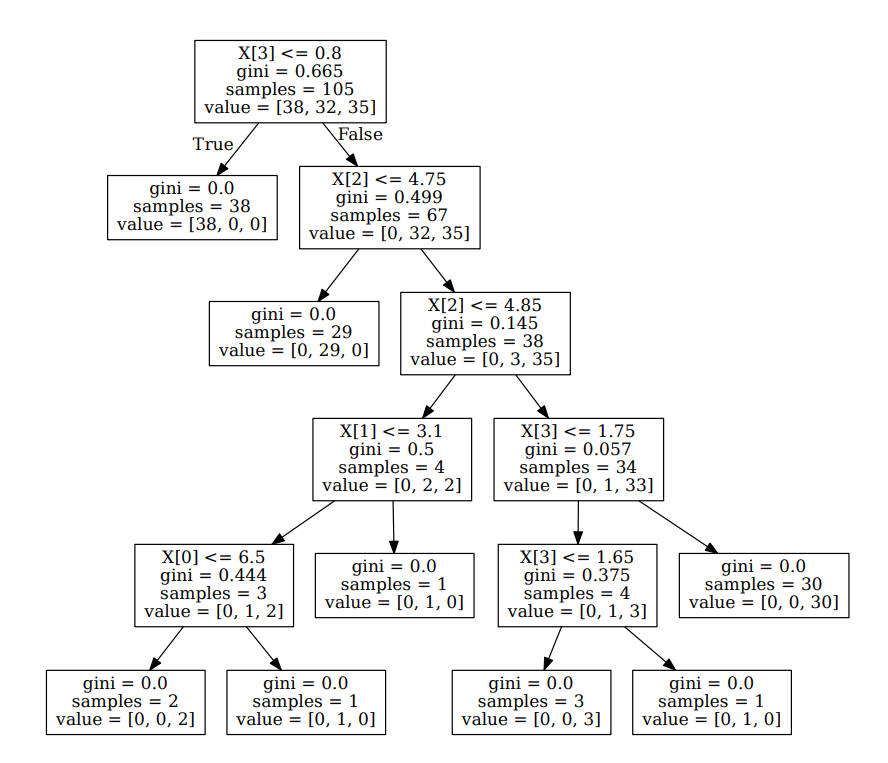
总结

通过可视化决策树，可以看出正如前面介绍的那样，分类决策树是 if-then 的集合，最终得到对应的分类结果。

波士顿房价之回归问题

在二手房产交易中，其中最受关注的便是房屋价格问题，其涉及到多个方方面面，例如房屋面积、房屋位置、户型大小、户型面积、小区平均房屋价格等等信息。现在 sklearn 提供波士顿的房屋价格数据集，其中有 506 例记录，包含城镇人均犯罪率、住宅用地比例、平均房间数等特征信息，学习使用这些信息准确预测波士顿的房屋价格，之后以此类推收集想要购买区域的房屋价格信息，就可以预测自身购买房屋价格是否划算。

波士顿房价数据集数据含义如下：

特征列名称	特征含义
CRIM	城镇人均犯罪率
ZN	占地面积超过25,000平方英尺的住宅用地比例
INDUS	每个城镇非零售业务的比例
CHAS	Charles River虚拟变量
NOX	一氧化氮浓度（每千万份）
RM	每间住宅的平均房间数
AGE	1940年以前建造的自住单位比例
DIS	波士顿的五个就业中心加权距离
RAD	径向高速公路的可达性指数
TAX	每10,000美元的全额物业税率
PTRATIO	城镇的学生与教师比例
B	1000*(Bk / 0.63)^2 其中Bk是城镇黑人的比例
LSTAT	区域中被认为是低收入阶层的比率
MEDV	自有住房的中位数报价, 单位1000美元

加载数据

# 1. 加载数据boston = pd.read_csv('./data/housing-3.csv')
boston.head()

	CRIM	ZN	INDUS	NOX	RM	AGE	DIS	RAD	TAX	PIRATIO	B	LSTAT	MEDV
0	0.00632	18.0	2.31	0.538	6.575	65.2	4.0900	1	296.0	15.3	396.90	4.98	24.0
1	0.02731	0.0	7.07	0.469	6.421	78.9	4.9671	2	242.0	17.8	396.90	9.14	21.6
2	0.02729	0.0	7.07	0.469	7.185	61.1	4.9671	2	242.0	17.8	392.83	4.03	34.7
3	0.03237	0.0	2.18	0.458	6.998	45.8	6.0622	3	222.0	18.7	394.63	2.94	33.4
4	0.06905	0.0	2.18	0.458	7.147	54.2	6.0622	3	222.0	18.7	396.90	5.33	36.2

预处理数据

# 2. 获取特征集和房价
x = boston.drop(['MEDV'], axis=1)
y = boston['MEDV']
x.head(), y.head()

(      CRIM    ZN  INDUS  CHAS    NOX     RM   AGE     DIS  RAD    TAX  \0  0.00632  18.0   2.31     0  0.538  6.575  65.2  4.0900    1  296.0   1  0.02731   0.0   7.07     0  0.469  6.421  78.9  4.9671    2  242.0   2  0.02729   0.0   7.07     0  0.469  7.185  61.1  4.9671    2  242.0   3  0.03237   0.0   2.18     0  0.458  6.998  45.8  6.0622    3  222.0   4  0.06905   0.0   2.18     0  0.458  7.147  54.2  6.0622    3  222.0   PIRATIO       B  LSTAT  0     15.3  396.90   4.98  1     17.8  396.90   9.14  2     17.8  392.83   4.03  3     18.7  394.63   2.94  4     18.7  396.90   5.33  ,0    24.01    21.62    34.73    33.44    36.2Name: MEDV, dtype: float64)

# 3. 测试集与训练集 7:3x_train, x_test, y_train, y_test = train_test_split(x, y, test_size=0.33)
x_train.head(), x_test.head(), y_train.head(), y_test.head()

(         CRIM    ZN  INDUS  CHAS    NOX     RM    AGE     DIS  RAD    TAX  \492   0.11132   0.0  27.74     0  0.609  5.983   83.5  2.1099    4  711.0   266   0.78570  20.0   3.97     0  0.647  7.014   84.6  2.1329    5  264.0   91    0.03932   0.0   3.41     0  0.489  6.405   73.9  3.0921    2  270.0   379  17.86670   0.0  18.10     0  0.671  6.223  100.0  1.3861   24  666.0   89    0.05302   0.0   3.41     0  0.489  7.079   63.1  3.4145    2  270.0   PIRATIO       B  LSTAT  492     20.1  396.90  13.35  266     13.0  384.07  14.79  91      17.8  393.55   8.20  379     20.2  393.74  21.78  89      17.8  396.06   5.70  ,CRIM    ZN  INDUS  CHAS    NOX     RM   AGE     DIS  RAD    TAX  \399  9.91655   0.0  18.10     0  0.693  5.852  77.8  1.5004   24  666.0   305  0.05479  33.0   2.18     0  0.472  6.616  58.1  3.3700    7  222.0   131  1.19294   0.0  21.89     0  0.624  6.326  97.7  2.2710    4  437.0   452  5.09017   0.0  18.10     0  0.713  6.297  91.8  2.3682   24  666.0   121  0.07165   0.0  25.65     0  0.581  6.004  84.1  2.1974    2  188.0   PIRATIO       B  LSTAT  399     20.2  338.16  29.97  305     18.4  393.36   8.93  131     21.2  396.90  12.26  452     20.2  385.09  17.27  121     19.1  377.67  14.27  ,492    20.1266    30.791     22.0379    10.289     28.7Name: MEDV, dtype: float64,399     6.3305    28.4131    19.6452    16.1121    20.3Name: MEDV, dtype: float64)

训练回归模型

# 4. 创建 CART 回归树dtr = DecisionTreeRegressor()

# 5. 训练构造 CART 回归树dtr.fit(x_train, y_train)

DecisionTreeRegressor()

DecisionTreeRegressor?Documentation for DecisionTreeRegressoriFitted

DecisionTreeRegressor()

# 6. 预测测试集中的房价y_pred = dtr.predict(x_test)
y_pred

array([ 7.5, 28.7, 19.2, 16.7, 22. , 26.6, 21. , 15. , 13.2, 23.2,  8.8,25. , 13.8, 30.7, 32. , 13.3, 22.9, 19.6, 22.7,  8.8, 19.9, 15.6,7.5, 11.7, 36.2, 28.1, 17. , 20.2, 14.9, 25. , 20.2, 27.1, 17.5,36. , 14.9,  9.5, 23. , 16.7, 24.8, 20. , 20. ,  8.3, 31.6, 14.1,23.7, 19.4, 33.4, 29.6, 14.1, 22. , 23.1, 50. , 50. ,  8.3, 11.8,21. , 27.5, 15.2, 20. , 18.3,  8.3, 20.1, 17.6, 18.5, 32. , 17. ,19.9, 18.8, 11.7, 25. , 16. , 26.4, 32.7, 20.6, 50. , 14.4, 34.6,11.8, 20.1, 22.4, 28.6, 36.4, 12.6, 19.8, 34.6, 22.9,  5. , 33.1,50. , 20.3, 26.7, 18.2, 28.1, 44.8, 50. , 16. , 26.4, 23.2, 22.2,12. ,  8.3, 18.2, 19.6, 21.6, 11.9, 18.3, 28.1, 24.7, 22. , 32.5,20.6, 16.6, 18.2, 14.1, 20.5, 22. , 22.9,  7.5, 16.6, 19.9, 18.7,27.9, 23.2, 17.2, 23.8, 22.2, 20.9, 13.6, 19.3,  9.5, 27.9,  7.5,34.6, 13.8,  8.3, 50. , 10.2, 12.6, 32. , 24.2, 17. , 19.5, 23.7,24.3, 13.6, 22.6,  8.3, 23.1, 21.6, 24.5, 14. , 23.3, 24.4, 16.6,14.9, 22. ,  8.3, 19.9, 12.6, 10.2, 23.4, 24.7, 50. , 19.4, 20. ,14.3, 23. ])

计算测试集指标

# 7. 测试集结果评价
from sklearn.metrics import r2_score, mean_squared_error, mean_absolute_error# r2_score 决定系数，反映因变量的全部变异能通过回归关系被自变量解释的比例。
r2 = r2_score(y_test, y_pred)
mse = mean_squared_error(y_test, y_pred)
# 计算均值绝对误差 (MAE)
mae = mean_absolute_error(y_test, y_pred)
r2, mse, mae

(0.6862919611706397, 22.763832335329337, 3.143712574850299)

闯关题

STEP1：请根据要求完成题目

Q1. iris数据集中共有四个特征，重要性最小的特征是哪个？
A. 花萼长度
B. 花萼宽度
C. 花瓣长度
D. 花瓣宽度

a1 = 'A'

# 获取数据集描述
print(iris.DESCR)

.. _iris_dataset:Iris plants dataset
--------------------**Data Set Characteristics:**:Number of Instances: 150 (50 in each of three classes)
:Number of Attributes: 4 numeric, predictive attributes and the class
:Attribute Information:- sepal length in cm- sepal width in cm- petal length in cm- petal width in cm- class:- Iris-Setosa- Iris-Versicolour- Iris-Virginica:Summary Statistics:============== ==== ==== ======= ===== ====================Min  Max   Mean    SD   Class Correlation
============== ==== ==== ======= ===== ====================
sepal length:   4.3  7.9   5.84   0.83    0.7826
sepal width:    2.0  4.4   3.05   0.43   -0.4194
petal length:   1.0  6.9   3.76   1.76    0.9490  (high!)
petal width:    0.1  2.5   1.20   0.76    0.9565  (high!)
============== ==== ==== ======= ===== ====================:Missing Attribute Values: None
:Class Distribution: 33.3% for each of 3 classes.
:Creator: R.A. Fisher
:Donor: Michael Marshall (MARSHALL%PLU@io.arc.nasa.gov)
:Date: July, 1988The famous Iris database, first used by Sir R.A. Fisher. The dataset is taken
from Fisher's paper. Note that it's the same as in R, but not as in the UCI
Machine Learning Repository, which has two wrong data points.This is perhaps the best known database to be found in the
pattern recognition literature.  Fisher's paper is a classic in the field and
is referenced frequently to this day.  (See Duda & Hart, for example.)  The
data set contains 3 classes of 50 instances each, where each class refers to a
type of iris plant.  One class is linearly separable from the other 2; the
latter are NOT linearly separable from each other... dropdown:: References- Fisher, R.A. "The use of multiple measurements in taxonomic problems"Annual Eugenics, 7, Part II, 179-188 (1936); also in "Contributions toMathematical Statistics" (John Wiley, NY, 1950).- Duda, R.O., & Hart, P.E. (1973) Pattern Classification and Scene Analysis.(Q327.D83) John Wiley & Sons.  ISBN 0-471-22361-1.  See page 218.- Dasarathy, B.V. (1980) "Nosing Around the Neighborhood: A New SystemStructure and Classification Rule for Recognition in Partially ExposedEnvironments".  IEEE Transactions on Pattern Analysis and MachineIntelligence, Vol. PAMI-2, No. 1, 67-71.- Gates, G.W. (1972) "The Reduced Nearest Neighbor Rule".  IEEE Transactionson Information Theory, May 1972, 431-433.- See also: 1988 MLC Proceedings, 54-64.  Cheeseman et al"s AUTOCLASS IIconceptual clustering system finds 3 classes in the data.- Many, many more ...