python计算机视觉编程——9.图像分割
- 9.图像分割
- 9.1 图割
- 安装Graphviz
- 下一步:正文
- 9.1.1 从图像创建图
- 9.1.2 用户交互式分割
- 9.2 利用聚类进行分割
- 9.3 变分法
9.图像分割
9.1 图割
可以选择不装Graphviz,因为原本觉得是要用,后面发现好像用不到。不安装可直接跳到下一步
安装Graphviz
-
首先需要先下载Graphviz软件(Download | Graphviz),那些包先不要下载,网上说先下载包再下载软件会报错。在安装过程中,需要注意下图中的一步,其余都是一直下一步就行

-
检查一下环境变量的路径

-
接着在自己创建的虚拟环境下安装包
pip install pydotpluspip install graphviz -
这里需要注意的是,还需要再安装一个包,否则单单安装上面的会报错
pip install python-graphviz -
测试代码
from graphviz import Digraph
dot = Digraph(comment='The Round Table')
dot.node('A', 'King Arthur')
dot.node('B', 'Sir Bedevere the Wise')
dot.node('L', 'Sir Lancelot the Brave')dot.edges(['AB', 'AL'])
dot.edge('B', 'L', constraint='false')
print(dot.source)  dot.render('round-table.gv',format='jpg', view=True)

下一步:正文
- 图割:将一个有向图分割成两个互不相交的集合
- 基本思想:相似且彼此相近的像素应该划分到同一区域
图割C(C是图中所有边的集合)的“代价”函数定义为所有割的边的权重求合相加:
E c u t = ∑ ( i , j ) ∈ C w i j E_{cut}=\sum_{(i,j)\in C}w_{ij} Ecut=(i,j)∈C∑wij
w i j w_{ij} wij是图中节点i到节点j的边 ( i , j ) (i,j) (i,j)的权重,并且是对割C所有的边进行求和
我们需要用图来表示图像,并对图进行划分,以使得 E c u t E_{cut} Ecut最小。同时在用图表示图像时,需要额外增加两个节点(源点和汇点),并仅考虑那些将源点和汇点分开的割
寻找最小割等同于在源点和汇点间寻找最大流,这里需要用到python-graph工具包( 注:不是 p i p 下载 ! \color{red}{注:不是pip下载!} 注:不是pip下载!),工具包地址如下:GitHub - pmatiello/python-graph: New official repository: https://github.com/Shoobx/python-graph
下载完后,把文件夹放入导包的根目录

根据路径进行引包,如果引入没有报错,就说明没有问题
from python_graph.core.pygraph.classes.digraph import digraph
from python_graph.core.pygraph.algorithms.minmax import maximum_flow``
这里我是报错了:“jaraco.text"中没有drop_comment, join_continuation, yield_lines函数的问题,然后我在”_jaraco_text.py"文件里找到了这三个函数,索性就直接把他提到根目录上,发现就没报错了


另一个导包路径错误在"digraph.py"和"minmax.py"文件中

接着就可以运行代码了
gr = digraph()
gr.add_nodes([0,1,2,3])
gr.add_edge((0,1), wt=4)
gr.add_edge((1,2), wt=3)
gr.add_edge((2,3), wt=5)
gr.add_edge((0,2), wt=3)
gr.add_edge((1,3), wt=4)
flows,cuts = maximum_flow(gr,0,3)
print('flow is:', flows)
print('cut is:', cuts)

9.1.1 从图像创建图
我们需要利用图像像素作为节点定义一个图,除了像素节点外,还有两个特定的节点——“源”点和“汇”点,来分别代表图像的前景和背景,我们需要做的是将所有像素与源点、汇点链接起来。
- 每个像素节点都有一个从源点的传入边
- 每个像素节点都有一个到汇点的传出边
- 每个像素节点都有一条传入边和传出边连接到它的近邻。
接着需要用朴素贝叶斯分类器进行分类,我们将第8章的BayesClassifier类搬过来
def build_bayes_graph(im,labels,sigma=1e2,kappa=1):""" 从像素四邻域建立一个图,前景和背景(前景用1标记,背景用-1标记,其他的用0标记)由labels决定,并用朴素贝叶斯分类器建模"""m,n = im.shape[:2]# 每行是一个像素的RGB向量vim = im.reshape((-1,3))# 前景和背景(RGB)foreground = im[labels==1].reshape((-1,3))background = im[labels==-1].reshape((-1,3)) train_data = [foreground,background]# 训练朴素贝叶斯分类器bc = BayesClassifier()bc.train(train_data)# 获取所有像素的概率bc_lables,prob = bc.classify(vim)prob_fg = prob[0]prob_bg = prob[1]# 用m*n+2 个节点创建图gr = digraph()gr.add_nodes(range(m*n+2))source = m*n # 倒数第二个是源点sink = m*n+1 # 最后一个节点是汇点# 归一化for i in range(vim.shape[0]):vim[i] = vim[i] / (np.linalg.norm(vim[i]) + 1e-9)# go through all nodes and add edgesfor i in range(m*n):# 从源点添加边gr.add_edge((source,i),wt=prob_fg[i]/(prob_fg[i]+prob_bg[i]))# 向汇点添加边gr.add_edge((i,sink),wt=prob_bg[i]/(prob_fg[i]+prob_bg[i]))# 向相邻节点添加边if i%n != 0: # 左边存在edge_wt = kappa*np.exp(-1.0*sum((vim[i]-vim[i-1])**2)/sigma)gr.add_edge((i,i-1),wt=edge_wt)if (i+1)%n != 0: # 如果右边存在edge_wt = kappa*np.exp(-1.0*sum((vim[i]-vim[i+1])**2)/sigma)gr.add_edge((i,i+1),wt=edge_wt)if i//n != 0: # 如果上方存在edge_wt = kappa*np.exp(-1.0*sum((vim[i]-vim[i-n])**2)/sigma)gr.add_edge((i,i-n),wt=edge_wt)if i//n != m-1: # 如果下方存在edge_wt = kappa*np.exp(-1.0*sum((vim[i]-vim[i+n])**2)/sigma)gr.add_edge((i,i+n),wt=edge_wt)return gr
def gauss(m,v,x):""" Evaluate Gaussian in d-dimensions with independent mean m and variance v at the points in (the rows of) x. http://en.wikipedia.org/wiki/Multivariate_normal_distribution """if len(x.shape)==1:n,d = 1,x.shape[0]else:n,d = x.shape# covariance matrix, subtract meanS = np.diag(1/v)x = x-m# product of probabilitiesy = np.exp(-0.5*np.diag(np.dot(x,np.dot(S,x.T))))# normalize and returnreturn y * (2*np.pi)**(-d/2.0) / (np.sqrt(np.prod(v)) + 1e-6)
写入新函数
def build_bayes_graph(im,labels,sigma=1e2,kappa=1):""" 从像素四邻域建立一个图,前景和背景(前景用1标记,背景用-1标记,其他的用0标记)由labels决定,并用朴素贝叶斯分类器建模"""m,n = im.shape[:2]# 每行是一个像素的RGB向量vim = im.reshape((-1,3))# 前景和背景(RGB)foreground = im[labels==1].reshape((-1,3))background = im[labels==-1].reshape((-1,3)) train_data = [foreground,background]# 训练朴素贝叶斯分类器bc = BayesClassifier()bc.train(train_data)# 获取所有像素的概率bc_lables,prob = bc.classify(vim)prob_fg = prob[0]prob_bg = prob[1]# 用m*n+2 个节点创建图gr = nx.DiGraph()nodes=[]for i in range(m*n+2):nodes.append(str(i))gr.add_nodes_from(nodes)source = m*n # 倒数第二个是源点sink = m*n+1 # 最后一个节点是汇点# 归一化for i in range(vim.shape[0]):vim[i] = vim[i] / (np.linalg.norm(vim[i]) + 1e-9)# go through all nodes and add edgesfor i in range(m*n):# 从源点添加边gr.add_edge(str(source),str(i),capacity=prob_fg[i]/(prob_fg[i]+prob_bg[i]))# 向汇点添加边gr.add_edge(str(i),str(sink),capacity=prob_bg[i]/(prob_fg[i]+prob_bg[i]))# 向相邻节点添加边if i%n != 0: # 左边存在edge_wt = kappa*np.exp(-1.0*sum((vim[i]-vim[i-1])**2)/sigma)gr.add_edge(str(i),str(i-1),capacity=edge_wt)if (i+1)%n != 0: # 如果右边存在edge_wt = kappa*np.exp(-1.0*sum((vim[i]-vim[i+1])**2)/sigma)gr.add_edge(str(i),str(i+1),capacity=edge_wt)if i//n != 0: # 如果上方存在edge_wt = kappa*np.exp(-1.0*sum((vim[i]-vim[i-n])**2)/sigma)gr.add_edge(str(i),str(i-n),capacity=edge_wt)if i//n != m-1: # 如果下方存在edge_wt = kappa*np.exp(-1.0*sum((vim[i]-vim[i+n])**2)/sigma)gr.add_edge(str(i),str(i+n),capacity=edge_wt)return gr
def show_labeling(im,labels):"""显示图像的前景和背景区域。前景labels=1,背景labels=-1,其他labels=0 """imshow(im)contour(labels,[-0.5,0.5])contourf(labels,[-1,-0.5],colors='b',alpha=0.25)contourf(labels,[0.5,1],colors='r',alpha=0.25)#axis('off')xticks([])yticks([])
def cut_graph(gr,imsize):"""    Solve max flow of graph gr and return binary labels of the resulting segmentation."""
#     print(gr)m,n=imsizesource=m*n # second to last is sourcesink=m*n+1 # last is sink# cut the graphflows,cuts = maximum_flow(gr,source,sink)
#     print(cuts)# convert graph to image with labelsres = np.zeros(m*n)for pos,label in list(cuts.items())[:-2]: # 遍历所有节点,忽略源节点和汇节点# 但因为cuts.items()返回的是元组,需先转成列表再进行切片res[pos] = labelreturn res.reshape((m,n))
其中书本中from scipy.misc import imresize模块,已经不存在于imresize中,这里使用Pillow库中的resize函数进行替代 resize_image_pillow
def resize_image_pillow(image_path, output_path, scale_factor):# 打开图像文件with Image.open(image_path) as img:# 计算新的尺寸new_width = int(img.width * scale_factor)new_height = int(img.height * scale_factor)# 使用双线性插值调整图像大小img_resized = img.resize((new_width, new_height), resample=Image.BILINEAR)# 保存调整后的图像
#         return img_resizedimg_resized.save(output_path)
import numpy as np
from PIL import Image
from pylab import *# resize_image_pillow('empire.jpg', 'empire.jpg', 0.07)
im=np.array(Image.open('empire.jpg'))
size=im.shape[:2]
labels=np.zeros(size)
labels[3:18,3:18]=-1
labels[-18:-3,-18:-3]=1# 对图进行分割
g = build_bayes_graph(im,labels,kappa=1)
res=cut_graph(g,size)figure()
show_labeling(im,labels)figure()
imshow(res)
gray()
axis('off')show()

9.1.2 用户交互式分割
def create_msr_labels(m, lasso=False):""" Create label matrix for training fromuser annotations. """labels = np.zeros(im.shape[:2])# backgroundlabels[m == 0] = -1labels[m == 64] = -1# foregroundif lasso:labels[m == 255] = 1else:labels[m == 128] = 1return labels# load image and annotation map
im = array(Image.open('empire.jpg'))
m = array(Image.open('empire.bmp'))
# resize
scale = 0.1
im = imresize(im, scale, interp='bilinear')
m = imresize(m, scale, interp='nearest')
# create training labels
labels = create_msr_labels(m, False)
# build graph using annotations
g = build_bayes_graph(im, labels, kappa=2)# cut graph
res = cut_graph(g, im.shape[:2])
# remove parts in background
res[m == 0] = 1
res[m == 64] = 1# plot the result
figure()
imshow(res)
gray()
xticks([])
yticks([])
savefig('labelplot.pdf')
9.2 利用聚类进行分割
def ncut_graph_matrix(im,sigma_d=1e2,sigma_g=1e-2):""" 创建用于归一化割的矩阵,其中 sigma_d 和 sigma_g 是像素距离和像素相似性的权重参数 """m,n = im.shape[:2] N = m*n# 归一化,并创建 RGB 或灰度特征向量if len(im.shape)==3:for i in range(3):im[:,:,i] = im[:,:,i] / im[:,:,i].max()vim = im.reshape((-1,3))else:im = im / im.max()vim = im.flatten()# x,y 坐标用于距离计算xx,yy = meshgrid(range(n),range(m))x,y = xx.flatten(),yy.flatten()# 创建边线权重矩阵W = zeros((N,N),'f')for i in range(N):for j in range(i,N):d = (x[i]-x[j])**2 + (y[i]-y[j])**2 W[i,j] = W[j,i] = exp(-1.0*sum((vim[i]-vim[j])**2)/sigma_g) * exp(-d/sigma_d)return W
from scipy.cluster.vq import *
def cluster(S,k,ndim):""" 从相似性矩阵进行谱聚类 """# 检查对称性if sum(abs(S-S.T)) > 1e-10:print('not symmetric')# 创建拉普拉斯矩阵rowsum = sum(abs(S),axis=0)D = diag(1 / sqrt(rowsum + 1e-6))L = dot(D,dot(S,D))# 计算 L 的特征向量U,sigma,V = linalg.svd(L,full_matrices=False)# 从前 ndim 个特征向量创建特征向量# 堆叠特征向量作为矩阵的列features = array(V[:ndim]).T# k-meansfeatures = whiten(features)centroids,distortion = kmeans(features,k)code,distance = vq(features,centroids)return code,V
在运行下面代码之前,需要安装scikit-image,记得在自己的虚拟环境下安装(我用pip安装不了,后面改用conda,只要在虚拟环境下,用哪个(pip或conda)都是安装在虚拟环境下)
conda install scikit-image
import cv2
import numpy as np
from pylab import  *
from PIL import Image
from skimage.transform import resizeim = Image.open('empire.jpg')
m,n = np.array(im).shape[:2]
# 调整图像的尺寸大小为(wid,wid)
wid = 50rim = im.resize((50,50),Image.BILINEAR)
rim = array(rim,'f')
# 创建归一化割矩阵
# print(rim.shape[:2] )
A = ncut_graph_matrix(rim,sigma_d=1,sigma_g=1e-2)
# 聚类
code,V=cluster(A,k=3,ndim=3)
# 变换到原来的图像大小image=code.reshape(wid,wid)
print(image)codeim = resize(image,(m,n),mode='reflect',anti_aliasing=False,order=0)
# 绘制分割结果
figure()
imshow(codeim)
gray()
show()

9.3 变分法
当优化的对象是函数时,该问题称为变分问题,需要使用ROF进行降噪。
denoise函数需要传入以下参数
- im: 输入的噪声图像(灰度图像)。
- U_init: 对 U(去噪图像)的初始猜测。
- tolerance: 收敛的容忍度,用于判断迭代是否结束。
- tau: 步长(或称为步伐),用于控制更新的幅度。
- tv_weight: 总变差正则化项的权重,控制去噪程度。
denoise函数返回参数
- U: 去噪后的图像。
- im - U: 图像的纹理残差,即原始图像中未被去噪部分的残余。
def denoise(im,U_init,tolerance=0.1,tau=0.125,tv_weight=100):""" 这个函数实现了 Rudin-Osher-Fatemi (ROF) 去噪模型,ROF 模型是一个常用的图像去噪方法,基于总变差(Total Variation, TV)正则化来去除噪声,同时保留图像的边缘信息"""m,n=im.shape #获取图像的高度和宽度#初始化U=U_initPx=im # 对偶域的x分量Py=im # 对偶域的y分量error=1while(error>tolerance):Uold=U#原始变量的梯度GradUx=roll(U,-1,axis=1)-U #变量U梯度的x分量GradUy=roll(U,-1,axis=0)-U #变量U梯度的y分量#更新对偶变量PxNew=Px+(tau/tv_weight)*GradUx #更新PxPyNew=Py+(tau/tv_weight)*GradUy #更新PyNormNew=maximum(1,sqrt(PxNew**2+PyNew**2))#计算PxNew和PyNew的范数,确保其最小值为1Px=PxNew/NormNew #更新x分量Py=PyNew/NormNew #更新y分量RxPx=roll(Px,1,axis=1)#计算Px在x方向上的右移RyPy=roll(Py,1,axis=0)#计算Px在y方向上的下移DivP=(Px-RxPx)+(Py-RyPy)#计算Px和Py的梯度U=im+tv_weight*DivP # 更新去噪后的图像Uerror=linalg.norm(U-Uold)/sqrt(n*m)# 计算当前误差return U,im-U #返回去噪后的图像U和噪声图像
因为 scipy.misc.imsave 已被弃用,所以需要用其他库来完成,这里使用Pillow库来保存图像
import numpy as np
from PIL import Image
im = np.array(Image.open('ceramic-houses_t0.png').convert('L'))
U,T=denoise(im,im,tolerance=0.001)
t=0.4# 基于阈值生成二值图像
binary_image = U < t * U.max()# 将布尔数组转换为 uint8 格式(0 或 255)
binary_image_uint8 = (binary_image * 255).astype(np.uint8)# 创建 Image 对象
img = Image.fromarray(binary_image_uint8)# 保存图像为 PDF
img.save('result.pdf')
from pylab import  *
gray()
subplot(121)
imshow(U)
subplot(122)
imshow(img)