文章目录
- 前言
- PIECEWISE_JERK_PATH_OPTIMIZER功能简介
- PIECEWISE_JERK_PATH_OPTIMIZER相关配置
- PIECEWISE_JERK_PATH_OPTIMIZER总体流程
- OptimizePath
- piecewise_jerk_problem
- 二次规划问题标准形式
- 定义优化变量
- 定义目标函数
- 设计约束
- Optimize
- FormulateProblem计算QP系数矩阵
- CalculateKernel二次项系数P矩阵
- CalculateOffset一次项系数向量q
- CalculateAffineConstraint约束项系数A的矩阵\upper_bound\lower_bound
- SolverDefaultSettings 设定OSQP求解参数
- Else
- 参考
前言
在Apollo星火计划学习笔记——Apollo路径规划算法原理与实践与【Apollo学习笔记】——Planning模块讲到……Stage::Process的PlanOnReferenceLine函数会依次调用task_list中的TASK,本文将会继续以LaneFollow为例依次介绍其中的TASK部分究竟做了哪些工作。由于个人能力所限,文章可能有纰漏的地方,还请批评斧正。
在modules/planning/conf/scenario/lane_follow_config.pb.txt配置文件中,我们可以看到LaneFollow所需要执行的所有task。
stage_config: {stage_type: LANE_FOLLOW_DEFAULT_STAGEenabled: truetask_type: LANE_CHANGE_DECIDERtask_type: PATH_REUSE_DECIDERtask_type: PATH_LANE_BORROW_DECIDERtask_type: PATH_BOUNDS_DECIDERtask_type: PIECEWISE_JERK_PATH_OPTIMIZERtask_type: PATH_ASSESSMENT_DECIDERtask_type: PATH_DECIDERtask_type: RULE_BASED_STOP_DECIDERtask_type: SPEED_BOUNDS_PRIORI_DECIDERtask_type: SPEED_HEURISTIC_OPTIMIZERtask_type: SPEED_DECIDERtask_type: SPEED_BOUNDS_FINAL_DECIDERtask_type: PIECEWISE_JERK_SPEED_OPTIMIZER# task_type: PIECEWISE_JERK_NONLINEAR_SPEED_OPTIMIZERtask_type: RSS_DECIDER
本文将继续介绍LaneFollow的第5个TASK——PIECEWISE_JERK_PATH_OPTIMIZER
推荐阅读:Apollo星火计划学习笔记——Apollo路径规划算法原理与实践
PIECEWISE_JERK_PATH_OPTIMIZER功能简介
基于二次规划算法,对每个边界规划出最优路径.
PIECEWISE_JERK_PATH_OPTIMIZER相关配置
modules/planning/proto/task_config.proto
//
// PiecewiseJerkPathOptimizerConfigmessage PiecewiseJerkPathOptimizerConfig {optional PiecewiseJerkPathWeights default_path_config = 1;optional PiecewiseJerkPathWeights lane_change_path_config = 2;optional double path_reference_l_weight = 3 [default = 0.0];
}message PiecewiseJerkPathWeights {optional double l_weight = 1 [default = 1.0];optional double dl_weight = 2 [default = 100.0];optional double ddl_weight = 3 [default = 1000.0];optional double dddl_weight = 4 [default = 10000.0];
}
modules/planning/conf/planning_config.pb.txt
default_task_config: {task_type: PIECEWISE_JERK_PATH_OPTIMIZERpiecewise_jerk_path_optimizer_config {default_path_config {l_weight: 1.0dl_weight: 20.0ddl_weight: 1000.0dddl_weight: 50000.0}lane_change_path_config {l_weight: 1.0dl_weight: 5.0ddl_weight: 800.0dddl_weight: 30000.0}}
}
PIECEWISE_JERK_PATH_OPTIMIZER总体流程
输入:
const SpeedData& speed_data,const ReferenceLine& reference_line,const common::TrajectoryPoint& init_point,const bool path_reusable,PathData* const final_path_data
输出:
OptimizePath函数得到最优的路径,信息包括 o p t _ l , o p t _ d l , o p t _ d d l opt\_l,opt\_dl,opt\_ddl opt_l,opt_dl,opt_ddl。在Process函数中最终结果保存到了task基类的变量reference_line_info_中。
代码流程及框架
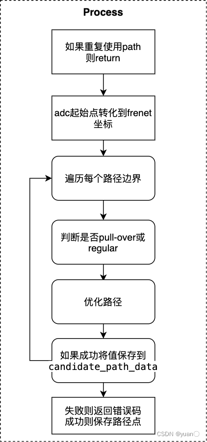
Process主要会调用OptimizePath()完成最优轨迹的求解、调用ToPiecewiseJerkPath()完成连续路径的离散化
common::Status PiecewiseJerkPathOptimizer::Process(const SpeedData& speed_data, const ReferenceLine& reference_line,const common::TrajectoryPoint& init_point, const bool path_reusable,PathData* const final_path_data) {// skip piecewise_jerk_path_optimizer if reused pathif (FLAGS_enable_skip_path_tasks && path_reusable) {return Status::OK();}ADEBUG << "Plan at the starting point: x = " << init_point.path_point().x()<< ", y = " << init_point.path_point().y()<< ", and angle = " << init_point.path_point().theta();common::TrajectoryPoint planning_start_point = init_point;if (FLAGS_use_front_axe_center_in_path_planning) {planning_start_point =InferFrontAxeCenterFromRearAxeCenter(planning_start_point);}// ADC起始点转化到frener坐标系const auto init_frenet_state =reference_line.ToFrenetFrame(planning_start_point);// Choose lane_change_path_config for lane-change cases// Otherwise, choose default_path_config for normal path planningconst auto& config = reference_line_info_->IsChangeLanePath()? config_.piecewise_jerk_path_optimizer_config().lane_change_path_config(): config_.piecewise_jerk_path_optimizer_config().default_path_config();// 根据选择的配置生成权重矩阵std::array<double, 5> w = {config.l_weight(),config.dl_weight() *std::fmax(init_frenet_state.first[1] * init_frenet_state.first[1],5.0),config.ddl_weight(), config.dddl_weight(), 0.0};// 获取路径边界const auto& path_boundaries =reference_line_info_->GetCandidatePathBoundaries();ADEBUG << "There are " << path_boundaries.size() << " path boundaries.";// 获取上一周期规划的path,做为此周期的参考pathconst auto& reference_path_data = reference_line_info_->path_data();// 遍历每个路径std::vector<PathData> candidate_path_data;for (const auto& path_boundary : path_boundaries) {size_t path_boundary_size = path_boundary.boundary().size();// if the path_boundary is normal, it is possible to have less than 2 points// skip path boundary of this kindif (path_boundary.label().find("regular") != std::string::npos &&path_boundary_size < 2) {continue;}int max_iter = 4000;// lower max_iter for regular/self/if (path_boundary.label().find("self") != std::string::npos) {max_iter = 4000;}CHECK_GT(path_boundary_size, 1U);std::vector<double> opt_l;std::vector<double> opt_dl;std::vector<double> opt_ddl;// 终止状态 l,dl,ddl = {0.0, 0.0, 0.0}std::array<double, 3> end_state = {0.0, 0.0, 0.0};// 判断是否处于pull over scenario,如果处于pull over scenario,调整end_stateif (!FLAGS_enable_force_pull_over_open_space_parking_test) {// pull over scenario// set end lateral to be at the desired pull over destinationconst auto& pull_over_status =injector_->planning_context()->planning_status().pull_over();if (pull_over_status.has_position() &&pull_over_status.position().has_x() &&pull_over_status.position().has_y() &&path_boundary.label().find("pullover") != std::string::npos) {common::SLPoint pull_over_sl;reference_line.XYToSL(pull_over_status.position(), &pull_over_sl);end_state[0] = pull_over_sl.l();}}// TODO(all): double-check this;// final_path_data might carry info from upper stream// 读取上一周期的 path_dataPathData path_data = *final_path_data;// updated cost function for path referencestd::vector<double> path_reference_l(path_boundary_size, 0.0);bool is_valid_path_reference = false;size_t path_reference_size = reference_path_data.path_reference().size();// 判断是否是regularif (path_boundary.label().find("regular") != std::string::npos &&reference_path_data.is_valid_path_reference()) {ADEBUG << "path label is: " << path_boundary.label();// when path reference is readyfor (size_t i = 0; i < path_reference_size; ++i) {common::SLPoint path_reference_sl;reference_line.XYToSL(common::util::PointFactory::ToPointENU(reference_path_data.path_reference().at(i).x(),reference_path_data.path_reference().at(i).y()),&path_reference_sl);path_reference_l[i] = path_reference_sl.l();}// 更新end_stateend_state[0] = path_reference_l.back();path_data.set_is_optimized_towards_trajectory_reference(true);is_valid_path_reference = true;}// 设置约束参数const auto& veh_param =common::VehicleConfigHelper::GetConfig().vehicle_param();const double lat_acc_bound =std::tan(veh_param.max_steer_angle() / veh_param.steer_ratio()) /veh_param.wheel_base();std::vector<std::pair<double, double>> ddl_bounds;for (size_t i = 0; i < path_boundary_size; ++i) {double s = static_cast<double>(i) * path_boundary.delta_s() +path_boundary.start_s();double kappa = reference_line.GetNearestReferencePoint(s).kappa();ddl_bounds.emplace_back(-lat_acc_bound - kappa, lat_acc_bound - kappa);}// 优化算法bool res_opt = OptimizePath(init_frenet_state, end_state, std::move(path_reference_l),path_reference_size, path_boundary.delta_s(), is_valid_path_reference,path_boundary.boundary(), ddl_bounds, w, max_iter, &opt_l, &opt_dl,&opt_ddl);// 如果成功将值保存到candidate_path_dataif (res_opt) {for (size_t i = 0; i < path_boundary_size; i += 4) {ADEBUG << "for s[" << static_cast<double>(i) * path_boundary.delta_s()<< "], l = " << opt_l[i] << ", dl = " << opt_dl[i];}auto frenet_frame_path =ToPiecewiseJerkPath(opt_l, opt_dl, opt_ddl, path_boundary.delta_s(),path_boundary.start_s());path_data.SetReferenceLine(&reference_line);path_data.SetFrenetPath(std::move(frenet_frame_path));if (FLAGS_use_front_axe_center_in_path_planning) {auto discretized_path = DiscretizedPath(ConvertPathPointRefFromFrontAxeToRearAxe(path_data));path_data.SetDiscretizedPath(discretized_path);}path_data.set_path_label(path_boundary.label());path_data.set_blocking_obstacle_id(path_boundary.blocking_obstacle_id());candidate_path_data.push_back(std::move(path_data));}}// 失败则返回错误码,成功则保存路径点if (candidate_path_data.empty()) {return Status(ErrorCode::PLANNING_ERROR,"Path Optimizer failed to generate path");}reference_line_info_->SetCandidatePathData(std::move(candidate_path_data));return Status::OK();
}
PS1:
// 设置约束参数const auto& veh_param =common::VehicleConfigHelper::GetConfig().vehicle_param();const double lat_acc_bound =std::tan(veh_param.max_steer_angle() / veh_param.steer_ratio()) /veh_param.wheel_base();std::vector<std::pair<double, double>> ddl_bounds;for (size_t i = 0; i < path_boundary_size; ++i) {double s = static_cast<double>(i) * path_boundary.delta_s() +path_boundary.start_s();double kappa = reference_line.GetNearestReferencePoint(s).kappa();ddl_bounds.emplace_back(-lat_acc_bound - kappa, lat_acc_bound - kappa);}
在这部分,我们主要关注lat_acc_bound和ddl_bounds两个参量。lat_acc_bound是根据车辆运动学关系计算最大曲率, α max \alpha_{\max} αmax是最大轮胎转向角(代码中应该是方向盘转角 δ \delta δ除以转向传动比): κ max = tan ( α max ) L {\kappa _{\max }} = \frac{{\tan ({\alpha _{\max }})}}{L} κmax=Ltan(αmax)
l ¨ \ddot l l¨的约束来源于这篇论文——Werling M, Ziegler J, Kammel S, et al. Optimal trajectory generation for dynamic street scenarios in a frenet frame[C]//2010 IEEE International Conference on Robotics and Automation. IEEE, 2010: 987-993.): d 2 l d s 2 = − ( κ r e f ′ l + κ r e f l ′ ) t a n ( θ − θ r e f ) + ( 1 − κ r e f l ) c o s 2 ( θ − θ r e f ) [ ( κ ( 1 − κ r e f l ) c o s ( θ − θ r e f ) − κ r e f ] \frac{d^2l}{ds^2}=-(\kappa_{ref}^{\prime}l+\kappa_{ref}l^{\prime})tan(\theta-\theta_{ref})+\frac{(1-\kappa_{ref}l)}{cos^2(\theta-\theta_{ref})}[\frac{(\kappa(1-\kappa_{ref}l)}{cos(\theta-\theta_{ref})}-\kappa_{ref}] ds2d2l=−(κref′l+κrefl′)tan(θ−θref)+cos2(θ−θref)(1−κrefl)[cos(θ−θref)(κ(1−κrefl)−κref]但我们无法直接将其应用于约束的设计(约束函数为一次)之中,对此需要对其进行简化。
假设1:参考线规划: θ − θ r e f = Δ θ ≈ 0 \theta - {\theta _{ref}} = \Delta \theta \approx 0 θ−θref=Δθ≈0,即航向角几乎为0.
假设2:规划的曲率数值上很小,所以两个曲率相乘近乎为0. 0 < κ r e f < κ ≪ 1 → κ r e f κ ≈ 0 0{\rm{ }} < {\kappa _{ref}} < \kappa \ll 1 \to {\kappa _{ref}}\kappa {\rm{ }} \approx {\rm{ }}0 0<κref<κ≪1→κrefκ≈0依据上述假设,我们将上述关系简化为: d 2 l d s 2 = κ − κ r e f \frac{{{d^2}l}}{{d{s^2}}} = \kappa - {\kappa _{ref}} ds2d2l=κ−κref
根据车辆运动学关系计算最大曲率 κ max {\kappa _{\max }} κmax,最后得到 l ¨ \ddot l l¨的约束范围:
− κ max − κ r e f < l ¨ i < κ max − κ r e f - {\kappa _{\max }} - {\kappa _{ref}} < {\ddot l_i} < {\kappa _{\max }} - {\kappa _{ref}} −κmax−κref<l¨i<κmax−κref
OptimizePath
路径优化算法在《Optimal Vehicle Path Planning Using Quadratic Optimization for Baidu Apollo Open Platform 》这篇论文中也有详细介绍,不过有些地方有些变化。
在OptimizePath会将PiecewiseJerkPathProblem实例化为piecewise_jerk_problem,进行以下优化过程。
1).定义piecewise_jerk_problem变量,优化算法
2).设置变量 a.权重 b.D方向距离、速度加速度边界 c.最大转角速度 d.jerk bound
3).优化算法 4).获取结果
OptimizePath函数是整个代码的核心部分。
首先来看一下相关的参数:
bool PiecewiseJerkPathOptimizer::OptimizePath(const std::pair<std::array<double, 3>, std::array<double, 3>>& init_state,const std::array<double, 3>& end_state,std::vector<double> path_reference_l_ref, const size_t path_reference_size,const double delta_s, const bool is_valid_path_reference,const std::vector<std::pair<double, double>>& lat_boundaries,const std::vector<std::pair<double, double>>& ddl_bounds,const std::array<double, 5>& w, const int max_iter, std::vector<double>* x,std::vector<double>* dx, std::vector<double>* ddx) {
init_state – path start point
end_state – path end point
path_reference_l_ref – a vector with default value 0.0
path_reference_size – length of learning model output
delta_s – path point spatial distance
is_valid_path_reference – whether using learning model output or not
lat_boundaries – path boundaries
ddl_bounds – constrains
w – weighting scales
max_iter – optimization max interations
ptr_x – optimization result of x
ptr_dx – optimization result of dx
ptr_ddx – optimization result of ddx
init_state初始状态点,end_state终末状态点,path_reference_l_ref参考线上各点的 l l l值,delta_s s s s方向的采样间隔。
在代码中,我们可以看到创建了一个PiecewiseJerkPathProblem类对象。接着来看一下与这个类相关的代码,文件路径在/modules/planning/math/piecewise_jerk下。
PiecewiseJerkPathProblem piecewise_jerk_problem(kNumKnots, delta_s,init_state.second);
.
├── BUILD
├── piecewise_jerk_path_problem.cc
├── piecewise_jerk_path_problem.h
├── piecewise_jerk_problem.cc
├── piecewise_jerk_problem.h
├── piecewise_jerk_speed_problem.cc
└── piecewise_jerk_speed_problem.h
可以看到该文件夹下包含三个类,piecewise_jerk_problem为基类,在这个基类中主要实现三个功能——整体最优化问题的框架、构造约束条件、求解二次优化问题。而piecewise_jerk_path_problem和piecewise_jerk_speed_problem则是这个基类的派生类,由此我们可以知道在Apollo中,path优化和speed优化的约束条件其实是一样的,都是在基类中实现的那个约束条件构造函数。而这两个派生类中又分别独自实现了代价函数的构造和一次项的构造这两个功能。
piecewise_jerk_problem
因此我们需要看看基类piecewise_jerk_problem具体的代码。
modules/planning/math/piecewise_jerk/piecewise_jerk_problem.cc
在此之前,我们需要了解一下二次规划的标准形式、路径优化所用的优化变量以及目标函数。
二次规划问题标准形式
二次规划问题的标准形式为: m i n i m i z e 1 2 x T P x + q T x s u b j e c t t o l ≤ A x ≤ u \begin{array}{lllllllllllllll}{{\rm{minimize}}}&{\frac{1}{2}{x^T}Px + {q^T}x}\\{{\rm{subject to}}}&{l \le Ax \le u}\end{array} minimizesubjectto21xTPx+qTxl≤Ax≤u where x ∈ R n x \in {{\bf{R}}^n} x∈Rn is the optimization variable. The objective function is defined by a positive semidefinite matrix P ∈ S + n P \in {\bf{S}}_ + ^n P∈S+nand vector q ∈ R n q \in {{\bf{R}}^n} q∈Rn . The linear constraints are defined by matrix A ∈ R m × n A \in {{\bf{R}}^{m \times n}} A∈Rm×n and vectors l l l and u u u so that l i ∈ R ∪ { − ∞ } {l_i} \in {\bf{R}} \cup \{ - \infty \} li∈R∪{−∞} and ‘ u i ∈ R ∪ { + ∞ } {`u_i} \in {\bf{R}} \cup \{ + \infty \} ‘ui∈R∪{+∞} for all i ∈ { 1 , … , m } i \in \{ 1, \ldots ,m{\rm{\} }} i∈{1,…,m} .
二次规划优化问题为二次型,其约束为线性型。 x x x是要优化的变量,是一个 n n n维的向量。 p p p是二次项系数,是正定矩阵。 q q q是一次项系数,是 n n n维向量。 A A A是一个 m m mx n n n的矩阵, A A A为约束函数的一次项系数, m m m为约束函数的个数。 l l l和 u u u分别为约束函数的下边界和上边界。
需要注意的是,二次规划只在代价函数为凸函数的时候能够收敛到最优解,因此这需要P矩阵为半正定矩阵,这是非常重要的一个条件。这反映在Apollo中的规划算法则为需要进行求解的空间为凸空间,这样二次规划才能收敛到一条最优path。
定义优化变量
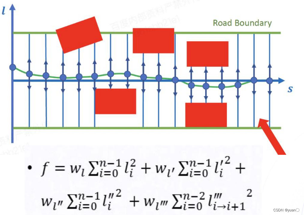
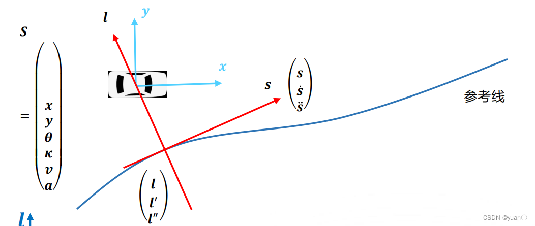 路径规划一般是在Frenet坐标系中进行的。 s s s为沿着参考线的方向, l l l为垂直于坐标系的方向。
 如图所示,将障碍物分别投影到SL坐标系上。在 s s s方向上,以间隔 Δ s \Delta s Δs作为一个间隔点,从 s 0 s_0 s0, s 1 s_1 s1, s 2 s_2 s2一直到 s n − 1 s_{n-1} sn−1,构成了规划的路径。选取每个间隔点的 l l l作为优化的变量,同时也将 l ˙ \dot l l˙和 l ¨ \ddot l l¨也作为优化变量。
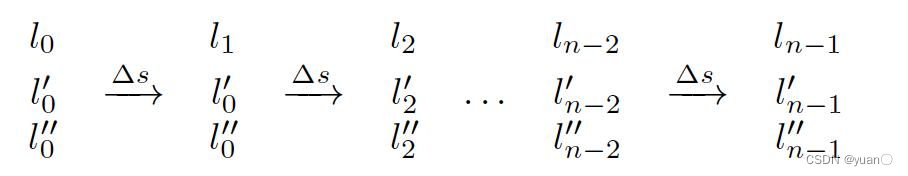 如此,就构成了优化变量 x x x, x x x有三个部分组成:从 l 0 l_0 l0, l 1 l_1 l1, l 2 l_2 l2到 l n − 1 l_{n-1} ln−1,从 l ˙ 0 \dot l_0 l˙0, l ˙ 1 \dot l_1 l˙1, l ˙ 2 \dot l_2 l˙2到 l ˙ n − 1 \dot l_{n-1} l˙n−1,从 l ¨ 0 \ddot l_0 l¨0, l ¨ 1 \ddot l_1 l¨1, l ¨ 2 \ddot l_2 l¨2到 l ¨ n − 1 \ddot l_{n-1} l¨n−1.
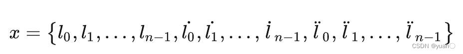
定义目标函数
对于目标函数的设计,我们需要明确以下目标:
- 确保安全、礼貌的驾驶,尽可能贴近车道中心线行驶: ∣ l i ∣ ↓ \left| {{l_i}} \right| \downarrow ∣li∣↓
- 确保舒适的体感,尽可能降低横向速度/加速度/加加速度: ∣ l ˙ i ∣ ↓ \left| {{{\dot l}_i}} \right| \downarrow l˙i ↓, ∣ l ¨ i ∣ ↓ \left| {{{\ddot l}_i}} \right| \downarrow l¨i ↓, ∣ l ′ ′ ′ i → i + 1 ∣ ↓ \left| {{{l'''}_{i \to i + 1}}} \right| \downarrow ∣l′′′i→i+1∣↓
- 确保终点接近参考终点(这个往往用在靠边停车场景之中国): l e n d = l r e f {l_{end}} = {l_{ref}} lend=lref
最后会得到以下目标函数:
m i n f = ∑ i = 0 n − 1 w l − r e f ( l i − l i − r e f ) 2 + w l l i 2 + w d l l i ˙ 2 + w d d l l ¨ i 2 + w d d d l l ( 3 ) i 2 + w e n d − l ( l n − 1 − l e n d − l ) 2 + w e n d − d l ( l n − 1 ˙ − l e n d − d l ) 2 + w e n d − d d l ( l n − 1 ¨ − l e n d − d d l ) 2 \begin{aligned} & minf=\sum_{i=0}^{n-1}w_{l-ref}(l_i-l_{i-ref})^2+w_l{l_i}^2+w_{dl}\dot{l_i}^2+w_{ddl}\ddot{l}_i^2+w_{dddl}{{l}^{(3)}}_i^2 \\ & +w_{end-l}(l_{n-1}-l_{end-l})^2+w_{end-dl}(\dot{l_{n-1}}-l_{end-dl})^2+w_{end-ddl}(\ddot{l_{n-1}}-l_{end-ddl})^2\end{aligned} minf=i=0∑n−1wl−ref(li−li−ref)2+wlli2+wdlli˙2+wddll¨i2+wdddll(3)i2+wend−l(ln−1−lend−l)2+wend−dl(ln−1˙−lend−dl)2+wend−ddl(ln−1¨−lend−ddl)2
对每个点设计二次的目标函数并对代价值进行求和,式中的 w l , w d l , w d d l , w d d d l {w_l},{w_{dl}},{w_{ddl}},{w_{dddl}} wl,wdl,wddl,wdddl都是对于优化变量的权重,以及偏移终点的权重 w e n d − l , w e n d − d l , w e n d − d d l , w e n d − d d d l {w_{end - l}},{w_{end - dl}},{w_{end - ddl}},{w_{end - dddl}} wend−l,wend−dl,wend−ddl,wend−dddl。
ps:三阶导的求解方式为: l ′ ′ i + 1 − l ′ ′ i Δ s \frac{{{{l''}_{i + 1}} - {{l''}_i}}}{{\Delta s}} Δsl′′i+1−l′′i
( l i ′ ′ ′ ) 2 = ( l i ′ ′ − l i − 1 ′ ′ Δ s ) 2 = ( l i ′ ′ ) 2 + ( l i − 1 ′ ′ ) 2 − 2 ⋅ l i ′ ′ ⋅ l i − 1 ′ ′ Δ s 2 \left(l_i^{\prime\prime\prime}\right)^2=\left(\frac{l_i^{\prime\prime}-l_{i-1}^{\prime\prime}}{\Delta s}\right)^2=\frac{\left(l_i^{\prime\prime}\right)^2+\left(l_{i-1}^{\prime\prime}\right)^2-2\cdot l_i^{\prime\prime}\cdot l_{i-1}^{\prime\prime}}{\Delta s^2} (li′′′)2=(Δsli′′−li−1′′)2=Δs2(li′′)2+(li−1′′)2−2⋅li′′⋅li−1′′
为了方便后续矩阵编写时查看,将目标函数按阶次整理如下:
min f = ∑ i = 0 n − 1 w l l i 2 + ∑ i = 0 n − 1 w l − r e f ( l i − l i − r e f ) 2 + w e n d − l ( l n − 1 − l e n d − d l ) 2 + ∑ i = 0 n − 1 w d l l i ′ 2 + w e n d − d l ( l n − 1 ′ − l e n d − d l ) 2 + ∑ i = 0 n − 1 w d d l l i ′ ′ 2 + w e n d − d d l ( l n − 1 ′ ′ − l e n d − d d l ) 2 + ∑ i = 0 n − 1 w d d d l l i ′ ′ ′ 2 \begin{aligned} \min f =& \sum_{i=0}^{n-1}{w_l}{l_i}^2 +\sum_{i=0}^{n-1} {{w_{l - ref}}} {({l_i} - {l_{i - ref}})^2} + {w_{end - l}}{( {{l_{n - 1}}} - {l_{end - dl}})^2}\\ +& \sum_{i=0}^{n-1}{w_{dl}}{ {{l_i}^{\prime}}^2} + {w_{end - dl}}{( {{l_{n - 1}}}^{\prime} - {l_{end - dl}})^2}\\ +& \sum_{i=0}^{n-1} {w_{ddl}}{{l_i}^{\prime\prime}}^2 +{w_{end - ddl}}{( {{l_{n - 1}}}^{\prime\prime} - {l_{end - ddl}})^2}\\ +& \sum_{i=0}^{n-1} {w_{dddl}}{{l_i}^{\prime\prime\prime}}^2 \end{aligned} minf=+++i=0∑n−1wlli2+i=0∑n−1wl−ref(li−li−ref)2+wend−l(ln−1−lend−dl)2i=0∑n−1wdlli′2+wend−dl(ln−1′−lend−dl)2i=0∑n−1wddlli′′2+wend−ddl(ln−1′′−lend−ddl)2i=0∑n−1wdddlli′′′2
再代入三阶导求解,可得(因为是用上下两个时刻的加速度算Jerk,所以只能得到n-1个Jerk):
∑ i = 1 n − 1 ( l i ′ ′ ′ ) 2 = ( l 1 ′ ′ − l 0 ′ ′ Δ s ) 2 + ( l 2 ′ ′ − l 1 ′ ′ Δ s ) 2 + ⋯ + ( l n − 2 ′ ′ − l n − 3 ′ ′ Δ s ) 2 + ( l n − 1 ′ ′ − l n − 2 ′ ′ Δ s ) 2 = ( l 0 ′ ′ ) 2 Δ s 2 + 2 ⋅ ∑ i = 1 n − 2 ( l i ′ ′ ) 2 Δ s 2 + ( l n − 1 ′ ′ ) 2 Δ s 2 − 2 ⋅ ∑ i = 0 n − 2 l i ′ ′ ⋅ l i + 1 ′ ′ Δ s 2 \begin{aligned} \sum_{\color{red}{i=1}}^{\color{red}{n-1}}(l_i^{\prime\prime\prime})^2& =\left(\frac{l_{1}^{\prime\prime}-l_{0}^{\prime\prime}}{\Delta s}\right)^2+\left(\frac{l_{2}^{\prime\prime}-l_{1}^{\prime\prime}}{\Delta s}\right)^2+\cdots+\left(\frac{l_{n-2}^{\prime\prime}-l_{n-3}^{\prime\prime}}{\Delta s}\right)^2+\left(\frac{l_{n-1}^{\prime\prime}-l_{n-2}^{\prime\prime}}{\Delta s}\right)^2 \\ &=\frac{\left(l_0^{\prime\prime}\right)^2}{\Delta s^2}+{2}\cdot\sum_{\color{red}i=1}^{\color{red}n-2}\frac{\left(l_i^{\prime\prime}\right)^2}{\Delta s^2}+\frac{\left(l_{n-1}^{\prime\prime}\right)^2}{\Delta s^2}-{2}\cdot\sum_{\color{red}i=0}^{\color{red}n-2}\frac{l_i^{\prime\prime}\cdot l_{i+1}^{\prime\prime}}{\Delta s^2} \end{aligned} i=1∑n−1(li′′′)2=(Δsl1′′−l0′′)2+(Δsl2′′−l1′′)2+⋯+(Δsln−2′′−ln−3′′)2+(Δsln−1′′−ln−2′′)2=Δs2(l0′′)2+2⋅i=1∑n−2Δs2(li′′)2+Δs2(ln−1′′)2−2⋅i=0∑n−2Δs2li′′⋅li+1′′
min f = ∑ i = 0 n − 1 w l l i 2 + ∑ i = 0 n − 1 w l − r e f ( l i − l i − r e f ) 2 + w e n d − l ( l n − 1 − l e n d − d l ) 2 + ∑ i = 0 n − 1 w d l l i ′ 2 + w e n d − d l ( l n − 1 ′ − l e n d − d l ) 2 + ∑ i = 0 n − 1 w d d l l i ′ ′ 2 + w e n d − d d l ( l n − 1 ′ ′ − l e n d − d d l ) 2 + w d d d l ⋅ [ ( l 0 ′ ′ ) 2 Δ s 2 + 2 ⋅ ∑ i = 1 n − 2 ( l i ′ ′ ) 2 Δ s 2 + ( l n − 1 ′ ′ ) 2 Δ s 2 − 2 ⋅ ∑ i = 0 n − 2 l i ′ ′ ⋅ l i + 1 ′ ′ Δ s 2 ] \begin{aligned} \min f =& \sum_{i=0}^{n-1}{w_l}{l_i}^2 +\sum_{i=0}^{n-1} {{w_{l - ref}}} {({l_i} - {l_{i - ref}})^2} + {w_{end - l}}{( {{l_{n - 1}}} - {l_{end - dl}})^2}\\ +& \sum_{i=0}^{n-1}{w_{dl}}{ {{l_i}^{\prime}}^2} + {w_{end - dl}}{( {{l_{n - 1}}}^{\prime} - {l_{end - dl}})^2}\\ +& \sum_{i=0}^{n-1} {w_{ddl}}{{l_i}^{\prime\prime}}^2 +{w_{end - ddl}}{( {{l_{n - 1}}}^{\prime\prime} - {l_{end - ddl}})^2}\\ +& {w_{dddl}}\cdot[\frac{\left(l_0^{\prime\prime}\right)^2}{\Delta s^2}+{2}\cdot\sum_{\color{red}i=1}^{\color{red}n-2}\frac{\left(l_i^{\prime\prime}\right)^2}{\Delta s^2}+\frac{\left(l_{n-1}^{\prime\prime}\right)^2}{\Delta s^2}-{2}\cdot\sum_{\color{red}i=0}^{\color{red}n-2}\frac{l_i^{\prime\prime}\cdot l_{i+1}^{\prime\prime}}{\Delta s^2}] \end{aligned} minf=+++i=0∑n−1wlli2+i=0∑n−1wl−ref(li−li−ref)2+wend−l(ln−1−lend−dl)2i=0∑n−1wdlli′2+wend−dl(ln−1′−lend−dl)2i=0∑n−1wddlli′′2+wend−ddl(ln−1′′−lend−ddl)2wdddl⋅[Δs2(l0′′)2+2⋅i=1∑n−2Δs2(li′′)2+Δs2(ln−1′′)2−2⋅i=0∑n−2Δs2li′′⋅li+1′′]
设计约束
接下来谈谈约束的设计,约束要满足:
• 主车必须在道路边界内,同时不能和障碍物有碰撞 l i ∈ ( l min i , l max i ) {l_i} \in (l_{\min }^i,l_{\max }^i) li∈(lmini,lmaxi)
• 根据当前状态,主车的横向速度/加速度/加加速度有特定运动学限制:
上文已经推导过 l ¨ \ddot l l¨的约束范围,接着推导三阶导的范围:
还得满足曲率变化率的要求(即规划处的路径能使方向盘在最大角速度下能够及时的转过来): d 3 l d s 3 = d d 2 t d l 2 d t ⋅ d t d s \frac{{{d^3}l}}{{d{s^3}}} = \frac{{d\frac{{{d^2}t}}{{d{l^2}}}}}{{dt}} \cdot \frac{{dt}}{{ds}} ds3d3l=dtddl2d2t⋅dsdt主路行驶中,实际车轮转角很小 α → 0 α→0 α→0,近似有 t a n α ≈ α tan α ≈ α tanα≈α,从而有: d 2 l d s 2 ≈ κ − κ r e f = tan ( α max ) L − κ r e f ≈ α L − κ r e f \frac{{{d^2}l}}{{d{s^2}}} \approx \kappa - {\kappa _{ref}} = \frac{{\tan ({\alpha _{\max }})}}{L} - {\kappa _{ref}} \approx \frac{\alpha }{L} - {\kappa _{ref}} ds2d2l≈κ−κref=Ltan(αmax)−κref≈Lα−κref同时假设,在一个周期内规划的路径上车辆的速度是恒定的 v = d s d t v = \frac{{ds}}{{dt}} v=dtds代入三阶导公式得到三阶导的边界 d 3 l d s 3 = α ′ L v < α ′ max L v \frac{{{d^3}l}}{{d{s^3}}} = \frac{{\alpha '}}{{Lv}} < \frac{{{{\alpha '}_{\max }}}}{{Lv}} ds3d3l=Lvα′<Lvα′max
总结一下横向速度/加速度/加加速度的约束:
l i ′ ∈ ( l m i n i ′ ( S ) , l m a x i ′ ( S ) ) , l i ′ ′ ∈ ( l m i n i ′ ′ ( S ) , l m a x i ′ ′ ( S ) ) , l i ′ ′ ′ ∈ ( l m i n i ′ ′ ′ ( S ) , l m a x i ′ ′ ′ ( S ) ) l_{i}^{\prime}\in\left(l_{min}^{i}{}^{\prime}(S),l_{max}^{i}{}^{\prime}(S)\right)\text{,}l_{i}^{\prime\prime}\in\left(l_{min}^{i}{}^{\prime\prime}(S),l_{max}^{i}{}^{\prime\prime}(S)\right)\text{,}l_{i}^{\prime\prime\prime}\in\left(l_{min}^{i}{}^{\prime\prime\prime}(S),l_{max}^{i}{}^{\prime\prime\prime}(S)\right) li′∈(lmini′(S),lmaxi′(S)),li′′∈(lmini′′(S),lmaxi′′(S)),li′′′∈(lmini′′′(S),lmaxi′′′(S))
• 连续性约束:
l i + 1 ′ ′ = l i ′ ′ + ∫ 0 Δ s l i → i + 1 ′ ′ ′ d s = l i ′ ′ + l i → i + 1 ′ ′ ′ ∗ Δ s l i + 1 ′ = l i ′ + ∫ 0 Δ s l ′ ′ ( s ) d s = l i ′ + l i ′ ′ ∗ Δ s + 1 2 ∗ l i → i + 1 ′ ′ ′ ∗ Δ s 2 = l i ′ + 1 2 ∗ l i ′ ′ ∗ Δ s + 1 2 ∗ l i + 1 ′ ′ ∗ Δ s l i + 1 = l i + ∫ 0 Δ s l ′ ( s ) d s = l i + l i ′ ∗ Δ s + 1 2 ∗ l i ′ ′ ∗ Δ s 2 + 1 6 ∗ l i → i + 1 ′ ′ ′ ∗ Δ s 3 = l i + l i ′ ∗ Δ s + 1 3 ∗ l i ′ ′ ∗ Δ s 2 + 1 6 ∗ l i + 1 ′ ′ ∗ Δ s 2 \begin{aligned} l_{i+1}^{\prime\prime} &=l_i''+\int_0^{\Delta s}l_{i\to i+1}^{\prime\prime\prime}ds=l_i''+l_{i\to i+1}^{\prime\prime\prime}*\Delta s \\ l_{i+1}^{\prime} &=l_i^{\prime}+\int_0^{\Delta s}\boldsymbol{l''}(s)ds=l_i^{\prime}+l_i^{\prime\prime}*\Delta s+\frac12*l_{i\to i+1}^{\prime\prime\prime}*\Delta s^2 \\ &= l_i^{\prime}+\frac12*l_i^{\prime\prime}*\Delta s+\frac12*l_{i+1}^{\prime\prime}*\Delta s\\ l_{i+1} &=l_i+\int_0^{\Delta s}\boldsymbol{l'}(s)ds \\ &=l_i+l_i^{\prime}*\Delta s+\frac12*l_i^{\prime\prime}*\Delta s^2+\frac16*l_{i\to i+1}^{\prime\prime\prime}*\Delta s^3\\ &=l_i+l_i^{\prime}*\Delta s+\frac13*l_i^{\prime\prime}*\Delta s^2+\frac16*l_{i+1}^{\prime\prime}*\Delta s^2 \end{aligned} li+1′′li+1′li+1=li′′+∫0Δsli→i+1′′′ds=li′′+li→i+1′′′∗Δs=li′+∫0Δsl′′(s)ds=li′+li′′∗Δs+21∗li→i+1′′′∗Δs2=li′+21∗li′′∗Δs+21∗li+1′′∗Δs=li+∫0Δsl′(s)ds=li+li′∗Δs+21∗li′′∗Δs2+61∗li→i+1′′′∗Δs3=li+li′∗Δs+31∗li′′∗Δs2+61∗li+1′′∗Δs2
• 起点的约束:
l 0 = l i n i t , l ˙ 0 = l i n i t , l ¨ 0 = l i n i t l_0=l_{init},\dot l_0=l_{init},\ddot l_0=l_{init} l0=linit,l˙0=linit,l¨0=linit
Optimize
在task中会调用Optimize进行路径优化。
// modules/planning/tasks/optimizers/piecewise_jerk_path/piecewise_jerk_path_optimizer.ccbool success = piecewise_jerk_problem.Optimize(max_iter);
Optimize函数中会调用FormulateProblem来构造出二次规划问题的框架,再调用osqp库进行求解,从而求出最优path。
求解器求解同样需要以下几个步骤:设定OSQP求解参数、计算QP系数矩阵、构造OSQP求解器、获取优化结果。
bool PiecewiseJerkProblem::Optimize(const int max_iter) {// 构造二次规划问题,计算QP系数矩阵OSQPData* data = FormulateProblem();// 设定OSQP求解参数OSQPSettings* settings = SolverDefaultSettings();settings->max_iter = max_iter;// 构造OSQP求解器OSQPWorkspace* osqp_work = nullptr;osqp_work = osqp_setup(data, settings);// osqp_setup(&osqp_work, data, settings);osqp_solve(osqp_work);// 获取优化值auto status = osqp_work->info->status_val;if (status < 0 || (status != 1 && status != 2)) {AERROR << "failed optimization status:\t" << osqp_work->info->status;osqp_cleanup(osqp_work);FreeData(data);c_free(settings);return false;} else if (osqp_work->solution == nullptr) {AERROR << "The solution from OSQP is nullptr";osqp_cleanup(osqp_work);FreeData(data);c_free(settings);return false;}// extract primal results//优化变量的取值x_.resize(num_of_knots_);dx_.resize(num_of_knots_);ddx_.resize(num_of_knots_);for (size_t i = 0; i < num_of_knots_; ++i) {x_.at(i) = osqp_work->solution->x[i] / scale_factor_[0];dx_.at(i) = osqp_work->solution->x[i + num_of_knots_] / scale_factor_[1];ddx_.at(i) =osqp_work->solution->x[i + 2 * num_of_knots_] / scale_factor_[2];}// Cleanuposqp_cleanup(osqp_work);FreeData(data);c_free(settings);return true;
}
FormulateProblem计算QP系数矩阵
OSQPData* PiecewiseJerkProblem::FormulateProblem() {// calculate kernelstd::vector<c_float> P_data;std::vector<c_int> P_indices;std::vector<c_int> P_indptr;// 二次项系数P的矩阵CalculateKernel(&P_data, &P_indices, &P_indptr);// calculate affine constraintsstd::vector<c_float> A_data;std::vector<c_int> A_indices;std::vector<c_int> A_indptr;std::vector<c_float> lower_bounds;std::vector<c_float> upper_bounds;// 约束项系数A的矩阵CalculateAffineConstraint(&A_data, &A_indices, &A_indptr, &lower_bounds,&upper_bounds);// calculate offsetstd::vector<c_float> q;// 一次项系数q的向量CalculateOffset(&q);OSQPData* data = reinterpret_cast<OSQPData*>(c_malloc(sizeof(OSQPData)));CHECK_EQ(lower_bounds.size(), upper_bounds.size());size_t kernel_dim = 3 * num_of_knots_;size_t num_affine_constraint = lower_bounds.size();data->n = kernel_dim;data->m = num_affine_constraint;data->P = csc_matrix(kernel_dim, kernel_dim, P_data.size(), CopyData(P_data),CopyData(P_indices), CopyData(P_indptr));data->q = CopyData(q);data->A =csc_matrix(num_affine_constraint, kernel_dim, A_data.size(),CopyData(A_data), CopyData(A_indices), CopyData(A_indptr));data->l = CopyData(lower_bounds);data->u = CopyData(upper_bounds);return data;
}
FormulateProblem 这个函数用于构造最优化问题具体矩阵。首先构造出P矩阵即代价函数,然后构造A矩阵即约束矩阵以及上下边界lower_bounds和upper_bounds,最后构建一次项q向量。构造完后将矩阵都存储进OSQPData这个结构体里,以便后续直接调用osqp库进行求解。
CalculateKernel二次项系数P矩阵
modules/planning/math/piecewise_jerk/piecewise_jerk_path_problem.cc
直接看路径优化部分P矩阵的构造。
void PiecewiseJerkSpeedProblem::CalculateKernel(std::vector<c_float>* P_data,std::vector<c_int>* P_indices,std::vector<c_int>* P_indptr) {const int n = static_cast<int>(num_of_knots_); // 待平滑的点数const int kNumParam = 3 * n;  // 待平滑的点数const int kNumValue = 4 * n - 1; // 非零元素的数目std::vector<std::vector<std::pair<c_int, c_float>>> columns; // 创建一个二维数组columns,用于存储每个变量对应的非零元素的索引和值columns.resize(kNumParam);int value_index = 0;// x(i)^2 * (w_x + w_x_ref[i]), w_x_ref might be a uniform value for all x(i)// or piecewise values for different x(i)for (int i = 0; i < n - 1; ++i) {columns[i].emplace_back(i, (weight_x_ + weight_x_ref_vec_[i]) /(scale_factor_[0] * scale_factor_[0]));++value_index;}// x(n-1)^2 * (w_x + w_x_ref[n-1] + w_end_x)columns[n - 1].emplace_back(n - 1, (weight_x_ + weight_x_ref_vec_[n - 1] + weight_end_state_[0]) /(scale_factor_[0] * scale_factor_[0]));++value_index;// x(i)'^2 * w_dxfor (int i = 0; i < n - 1; ++i) {columns[n + i].emplace_back(n + i, weight_dx_ / (scale_factor_[1] * scale_factor_[1]));++value_index;}// x(n-1)'^2 * (w_dx + w_end_dx)columns[2 * n - 1].emplace_back(2 * n - 1,(weight_dx_ + weight_end_state_[1]) /(scale_factor_[1] * scale_factor_[1]));++value_index;auto delta_s_square = delta_s_ * delta_s_;// x(i)''^2 * (w_ddx + 2 * w_dddx / delta_s^2)columns[2 * n].emplace_back(2 * n,(weight_ddx_ + weight_dddx_ / delta_s_square) /(scale_factor_[2] * scale_factor_[2]));++value_index;for (int i = 1; i < n - 1; ++i) {columns[2 * n + i].emplace_back(2 * n + i, (weight_ddx_ + 2.0 * weight_dddx_ / delta_s_square) /(scale_factor_[2] * scale_factor_[2]));++value_index;}columns[3 * n - 1].emplace_back(3 * n - 1,(weight_ddx_ + weight_dddx_ / delta_s_square + weight_end_state_[2]) /(scale_factor_[2] * scale_factor_[2]));++value_index;// -2 * w_dddx / delta_s^2 * x(i)'' * x(i + 1)''for (int i = 0; i < n - 1; ++i) {columns[2 * n + i].emplace_back(2 * n + i + 1,(-2.0 * weight_dddx_ / delta_s_square) /(scale_factor_[2] * scale_factor_[2]));++value_index;}CHECK_EQ(value_index, num_of_nonzeros);int ind_p = 0;for (int i = 0; i < num_of_variables; ++i) {P_indptr->push_back(ind_p);for (const auto& row_data_pair : columns[i]) {P_data->push_back(row_data_pair.second * 2.0);P_indices->push_back(row_data_pair.first);++ind_p;}}P_indptr->push_back(ind_p);
}scale_factor_[i]在上面代码中反复出现,应该是用以平衡不同阶导数之间的数量级的。
由于二次规划问题中P、A矩阵是稀疏的,为方便储存Apollo采用的是稀疏矩阵存储格式CSC(Compressed Sparse Column Format)。P_data,P_indices,P_indptr都是稀疏矩阵的参数,稀疏矩阵的具体形式可以看这篇博文【规划】Apollo QSQP接口详解。(稀疏矩阵这种形式确实不是很直观。)
最后,通过csc_matrix恢复稀疏矩阵。
data->P = csc_matrix(kernel_dim, kernel_dim, P_data.size(), CopyData(P_data),CopyData(P_indices), CopyData(P_indptr));
下面是 P P P矩阵
P = 2 ⋅ [ w l + w l − r e f 0 ⋯ 0 0 ⋱ ⋮ ⋮ w l + w l − r e f 0 0 ⋯ 0 w l + w l − r e f + w e n d − l w d l 0 ⋯ 0 0 ⋱ ⋮ ⋮ w d l 0 0 ⋯ 0 w d l + w e n d − d l w d d l + w d d d l Δ s 2 0 ⋯ ⋯ 0 − 2 ⋅ w d d d l Δ s 2 w d d l + 2 ⋅ w d d d l Δ s 2 ⋮ 0 − 2 ⋅ w d d d l Δ s 2 ⋱ ⋮ ⋮ ⋱ w d d l + 2 ⋅ w d d d l Δ s 2 0 0 ⋯ 0 − 2 ⋅ w d d d l Δ s 2 w d d l + w d d d l Δ s 2 + w e n d − d d l ] P=2\cdot\left[ {\begin{array}{ccccccccccccccc}{{\begin{array}{ccccccccccccccc}{{w_l} + {w_{l - ref}}}&0& \cdots &0\\0& \ddots &{}& \vdots \\ \vdots &{}&{{w_l} + {w_{l - ref}}}&0\\0& \cdots &0&{{w_l} + {w_{l - ref}} + {w_{end - l}}}\end{array}}}&{}&{}\\{}&{\begin{array}{ccccccccccccccc}{{w_{dl}}}&0& \cdots &0\\0& \ddots &{}& \vdots \\ \vdots &{}&{{w_{dl}}}&0\\0& \cdots &0&{{w_{dl}} + {w_{end - dl}}}\end{array}}&{}\\{}&{}&{\begin{array}{ccccccccccccccc}{{w_{ddl}} + \frac{{{w_{dddl}}}}{{\Delta {s^2}}}}&0& \cdots & \cdots &0\\{ - 2 \cdot \frac{{{w_{dddl}}}}{{\Delta {s^2}}}}&{{w_{ddl}} + 2 \cdot \frac{{{w_{dddl}}}}{{\Delta {s^2}}}}&{}&{}& \vdots \\0&{ - 2 \cdot \frac{{{w_{dddl}}}}{{\Delta {s^2}}}}& \ddots &{}& \vdots \\ \vdots &{}& \ddots &{{w_{ddl}} + 2 \cdot \frac{{{w_{dddl}}}}{{\Delta {s^2}}}}&0\\0& \cdots &0&{ - 2 \cdot \frac{{{w_{dddl}}}}{{\Delta {s^2}}}}&{{w_{ddl}} + \frac{{{w_{dddl}}}}{{\Delta {s^2}}} + {w_{end - ddl}}}\end{array}}\end{array}} \right] P=2⋅ wl+wl−ref0⋮00⋱⋯⋯wl+wl−ref00⋮0wl+wl−ref+wend−lwdl0⋮00⋱⋯⋯wdl00⋮0wdl+wend−dlwddl+Δs2wdddl−2⋅Δs2wdddl0⋮00wddl+2⋅Δs2wdddl−2⋅Δs2wdddl⋯⋯⋱⋱0⋯wddl+2⋅Δs2wdddl−2⋅Δs2wdddl0⋮⋮0wddl+Δs2wdddl+wend−ddl
CalculateOffset一次项系数向量q
void PiecewiseJerkPathProblem::CalculateOffset(std::vector<c_float>* q) {CHECK_NOTNULL(q);const int n = static_cast<int>(num_of_knots_);const int kNumParam = 3 * n;q->resize(kNumParam, 0.0);if (has_x_ref_) {for (int i = 0; i < n; ++i) {q->at(i) += -2.0 * weight_x_ref_vec_.at(i) * x_ref_[i] / scale_factor_[0];}}if (has_end_state_ref_) {q->at(n - 1) +=-2.0 * weight_end_state_[0] * end_state_ref_[0] / scale_factor_[0];q->at(2 * n - 1) +=-2.0 * weight_end_state_[1] * end_state_ref_[1] / scale_factor_[1];q->at(3 * n - 1) +=-2.0 * weight_end_state_[2] * end_state_ref_[2] / scale_factor_[2];}
}
一次项系数向量 q q q如下
q = [ − 2 ⋅ w l − r e f ⋅ l 0 − r e f ⋮ − 2 ⋅ w l − r e f ⋅ l ( n − 2 ) − r e f − 2 ⋅ w l − r e f ⋅ l ( n − 1 ) − r e f − 2 ⋅ w e n d − l ⋅ l e n d − l 0 ⋮ 0 − 2 ⋅ w e n d − d l ⋅ l e n d − d l 0 ⋮ 0 − 2 ⋅ w e n d − d d l ⋅ l e n d − d d l ] q = \left[ {\begin{array}{ccccccccccccccc}{ - 2 \cdot {w_{l - ref}} \cdot {l_{0 - ref}}}\\ \vdots \\{ - 2 \cdot {w_{l - ref}} \cdot {l_{(n - 2) - ref}}}\\{ - 2 \cdot {w_{l - ref}} \cdot {l_{(n - 1) - ref}} - {\rm{2}} \cdot {w_{end - l}} \cdot {l_{end - l}}}\\0\\ \vdots \\0\\{ - {\rm{2}} \cdot {w_{end - dl}} \cdot {l_{end - dl}}}\\0\\ \vdots \\0\\{ - {\rm{2}} \cdot {w_{end - ddl}} \cdot {l_{end - ddl}}}\end{array}} \right] q= −2⋅wl−ref⋅l0−ref⋮−2⋅wl−ref⋅l(n−2)−ref−2⋅wl−ref⋅l(n−1)−ref−2⋅wend−l⋅lend−l0⋮0−2⋅wend−dl⋅lend−dl0⋮0−2⋅wend−ddl⋅lend−ddl
CalculateAffineConstraint约束项系数A的矩阵\upper_bound\lower_bound
void PiecewiseJerkProblem::CalculateAffineConstraint(std::vector<c_float>* A_data, std::vector<c_int>* A_indices,std::vector<c_int>* A_indptr, std::vector<c_float>* lower_bounds,std::vector<c_float>* upper_bounds) {// 3N params bounds on x, x', x''// 3(N-1) constraints on x, x', x''// 3 constraints on x_init_const int n = static_cast<int>(num_of_knots_);const int num_of_variables = 3 * n;const int num_of_constraints = num_of_variables + 3 * (n - 1) + 3;lower_bounds->resize(num_of_constraints);upper_bounds->resize(num_of_constraints);std::vector<std::vector<std::pair<c_int, c_float>>> variables(num_of_variables);int constraint_index = 0;// set x, x', x'' boundsfor (int i = 0; i < num_of_variables; ++i) {if (i < n) {variables[i].emplace_back(constraint_index, 1.0);lower_bounds->at(constraint_index) =x_bounds_[i].first * scale_factor_[0];upper_bounds->at(constraint_index) =x_bounds_[i].second * scale_factor_[0];} else if (i < 2 * n) {variables[i].emplace_back(constraint_index, 1.0);lower_bounds->at(constraint_index) =dx_bounds_[i - n].first * scale_factor_[1];upper_bounds->at(constraint_index) =dx_bounds_[i - n].second * scale_factor_[1];} else {variables[i].emplace_back(constraint_index, 1.0);lower_bounds->at(constraint_index) =ddx_bounds_[i - 2 * n].first * scale_factor_[2];upper_bounds->at(constraint_index) =ddx_bounds_[i - 2 * n].second * scale_factor_[2];}++constraint_index;}CHECK_EQ(constraint_index, num_of_variables);// x(i->i+1)''' = (x(i+1)'' - x(i)'') / delta_sfor (int i = 0; i + 1 < n; ++i) {variables[2 * n + i].emplace_back(constraint_index, -1.0);variables[2 * n + i + 1].emplace_back(constraint_index, 1.0);lower_bounds->at(constraint_index) =dddx_bound_.first * delta_s_ * scale_factor_[2];upper_bounds->at(constraint_index) =dddx_bound_.second * delta_s_ * scale_factor_[2];++constraint_index;}// x(i+1)' - x(i)' - 0.5 * delta_s * x(i)'' - 0.5 * delta_s * x(i+1)'' = 0for (int i = 0; i + 1 < n; ++i) {variables[n + i].emplace_back(constraint_index, -1.0 * scale_factor_[2]);variables[n + i + 1].emplace_back(constraint_index, 1.0 * scale_factor_[2]);variables[2 * n + i].emplace_back(constraint_index,-0.5 * delta_s_ * scale_factor_[1]);variables[2 * n + i + 1].emplace_back(constraint_index,-0.5 * delta_s_ * scale_factor_[1]);lower_bounds->at(constraint_index) = 0.0;upper_bounds->at(constraint_index) = 0.0;++constraint_index;}// x(i+1) - x(i) - delta_s * x(i)'// - 1/3 * delta_s^2 * x(i)'' - 1/6 * delta_s^2 * x(i+1)''auto delta_s_sq_ = delta_s_ * delta_s_;for (int i = 0; i + 1 < n; ++i) {variables[i].emplace_back(constraint_index,-1.0 * scale_factor_[1] * scale_factor_[2]);variables[i + 1].emplace_back(constraint_index,1.0 * scale_factor_[1] * scale_factor_[2]);variables[n + i].emplace_back(constraint_index, -delta_s_ * scale_factor_[0] * scale_factor_[2]);variables[2 * n + i].emplace_back(constraint_index,-delta_s_sq_ / 3.0 * scale_factor_[0] * scale_factor_[1]);variables[2 * n + i + 1].emplace_back(constraint_index,-delta_s_sq_ / 6.0 * scale_factor_[0] * scale_factor_[1]);lower_bounds->at(constraint_index) = 0.0;upper_bounds->at(constraint_index) = 0.0;++constraint_index;}// constrain on x_initvariables[0].emplace_back(constraint_index, 1.0);lower_bounds->at(constraint_index) = x_init_[0] * scale_factor_[0];upper_bounds->at(constraint_index) = x_init_[0] * scale_factor_[0];++constraint_index;variables[n].emplace_back(constraint_index, 1.0);lower_bounds->at(constraint_index) = x_init_[1] * scale_factor_[1];upper_bounds->at(constraint_index) = x_init_[1] * scale_factor_[1];++constraint_index;variables[2 * n].emplace_back(constraint_index, 1.0);lower_bounds->at(constraint_index) = x_init_[2] * scale_factor_[2];upper_bounds->at(constraint_index) = x_init_[2] * scale_factor_[2];++constraint_index;CHECK_EQ(constraint_index, num_of_constraints);int ind_p = 0;for (int i = 0; i < num_of_variables; ++i) {A_indptr->push_back(ind_p);for (const auto& variable_nz : variables[i]) {// coefficientA_data->push_back(variable_nz.second);// constraint indexA_indices->push_back(variable_nz.first);++ind_p;}}// We indeed need this line because of// https://github.com/oxfordcontrol/osqp/blob/master/src/cs.c#L255A_indptr->push_back(ind_p);
}
l b = [ l l b [ 0 ] ⋮ l l b [ n − 1 ] l ′ l b [ 0 ] ⋮ l ′ l b [ n − 1 ] l ′ ′ l b [ 0 ] ⋮ l ′ ′ l b [ n − 1 ] l ′ ′ ′ l b [ 0 ] ⋅ Δ s ⋮ l ′ ′ ′ l b [ n − 2 ] ⋅ Δ s 0 ⋮ 0 l i n i t l ′ i n i t l ′ ′ i n i t ] , u b = [ l u b [ 0 ] ⋮ l u b [ n − 1 ] l ′ u b [ 0 ] ⋮ l ′ u b [ n − 1 ] l ′ ′ u b [ 0 ] ⋮ l ′ ′ u b [ n − 1 ] l ′ ′ ′ u b [ 0 ] ⋅ Δ s ⋮ l ′ ′ ′ u b [ n − 2 ] ⋅ Δ s 0 ⋮ 0 l i n i t l ′ i n i t l ′ ′ i n i t ] lb = \left[ {\begin{array}{ccccccccccccccc}{{l_{lb}}[0]}\\ \vdots \\{{l_{lb}}[n - 1]}\\{{{l'}_{lb}}[0]}\\ \vdots \\{{{l'}_{lb}}[n - 1]}\\{{{l''}_{lb}}[0]}\\ \vdots \\{{{l''}_{lb}}[n - 1]}\\{{{l'''}_{lb}}[0] \cdot \Delta s}\\ \vdots \\{{{l'''}_{lb}}[n - 2] \cdot \Delta s}\\0\\ \vdots \\0\\{{l_{init}}}\\{{{l'}_{init}}}\\{{{l''}_{init}}}\end{array}} \right],ub = \left[ {\begin{array}{ccccccccccccccc}{{l_{ub}}[0]}\\ \vdots \\{{l_{ub}}[n - 1]}\\{{{l'}_{ub}}[0]}\\ \vdots \\{{{l'}_{ub}}[n - 1]}\\{{{l''}_{ub}}[0]}\\ \vdots \\{{{l''}_{ub}}[n - 1]}\\{{{l'''}_{ub}}[0] \cdot \Delta s}\\ \vdots \\{{{l'''}_{ub}}[n - 2] \cdot \Delta s}\\0\\ \vdots \\0\\{{l_{init}}}\\{{{l'}_{init}}}\\{{{l''}_{init}}}\end{array}} \right] lb= llb[0]⋮llb[n−1]l′lb[0]⋮l′lb[n−1]l′′lb[0]⋮l′′lb[n−1]l′′′lb[0]⋅Δs⋮l′′′lb[n−2]⋅Δs0⋮0linitl′initl′′init ,ub= lub[0]⋮lub[n−1]l′ub[0]⋮l′ub[n−1]l′′ub[0]⋮l′′ub[n−1]l′′′ub[0]⋅Δs⋮l′′′ub[n−2]⋅Δs0⋮0linitl′initl′′init
PS:"0"的部分大小为2n-2。
A = [ 1 0 ⋯ 0 0 ⋱ ⋮ ⋮ ⋱ 0 0 ⋯ 0 1 1 0 ⋯ 0 0 ⋱ ⋮ ⋮ ⋱ 0 0 ⋯ 0 1 1 0 ⋯ 0 0 ⋱ ⋮ ⋮ ⋱ 0 0 ⋯ 0 1 − 1 1 ⋱ ⋱ − 1 1 − 1 1 ⋱ ⋱ − 1 1 − Δ s 2 − Δ s 2 ⋱ ⋱ − Δ s 2 − Δ s 2 − 1 1 ⋱ ⋱ − 1 1 − Δ s ⋱ − Δ s − Δ s 2 3 − Δ s 2 6 ⋱ ⋱ − Δ s 2 3 − Δ s 2 6 1 1 1 ] A = \left[ {\begin{array}{ccccccccccccccc}{\begin{array}{ccccccccccccccc}1&0& \cdots &0\\0& \ddots &{}& \vdots \\ \vdots &{}& \ddots &0\\0& \cdots &0&1\end{array}}&{}&{}\\{}&{\begin{array}{ccccccccccccccc}1&0& \cdots &0\\0& \ddots &{}& \vdots \\ \vdots &{}& \ddots &0\\0& \cdots &0&1\end{array}}&{}\\{}&{}&{\begin{array}{ccccccccccccccc}1&0& \cdots &0\\0& \ddots &{}& \vdots \\ \vdots &{}& \ddots &0\\0& \cdots &0&1\end{array}}\\{}&{}&{\begin{array}{ccccccccccccccc}{ - 1}&1&{}&{}\\{}& \ddots & \ddots &{}\\{}&{}&{ - 1}&1\end{array}}\\{}&{\begin{array}{ccccccccccccccc}{ - 1}&1&{}&{}\\{}& \ddots & \ddots &{}\\{}&{}&{ - 1}&1\end{array}}&{\begin{array}{ccccccccccccccc}{ - \frac{{\Delta s}}{2}}&{ - \frac{{\Delta s}}{2}}&{}&{}\\{}& \ddots & \ddots &{}\\{}&{}&{ - \frac{{\Delta s}}{2}}&{ - \frac{{\Delta s}}{2}}\end{array}}\\{\begin{array}{ccccccccccccccc}{ - 1}&1&{}&{}\\{}& \ddots & \ddots &{}\\{}&{}&{ - 1}&1\end{array}}&{\begin{array}{ccccccccccccccc}{ - \Delta s}&{}&{}&{}\\{}& \ddots &{}&{}\\{}&{}&{ - \Delta s}&{}\end{array}}&{\begin{array}{ccccccccccccccc}{ - \frac{{\Delta {s^2}}}{3}}&{ - \frac{{\Delta {s^2}}}{6}}&{}&{}\\{}& \ddots & \ddots &{}\\{}&{}&{ - \frac{{\Delta {s^2}}}{3}}&{ - \frac{{\Delta {s^2}}}{6}}\end{array}}\\{\begin{array}{ccccccccccccccc}1&{}&{}&{}\\{}&{}&{}&{}\\{}&{}&{}&{}\end{array}}&{\begin{array}{ccccccccccccccc}{}&{}&{}&{}\\1&{}&{}&{}\\{}&{}&{}&{}\end{array}}&{\begin{array}{ccccccccccccccc}{}&{}&{}&{}\\{}&{}&{}&{}\\1&{}&{}&{}\end{array}}\end{array}} \right] A= 10⋮00⋱⋯⋯⋱00⋮01−11⋱⋱−11110⋮00⋱⋯⋯⋱00⋮01−11⋱⋱−11−Δs⋱−Δs110⋮00⋱⋯⋯⋱00⋮01−11⋱⋱−11−2Δs−2Δs⋱⋱−2Δs−2Δs−3Δs2−6Δs2⋱⋱−3Δs2−6Δs21
SolverDefaultSettings 设定OSQP求解参数
OSQPSettings* PiecewiseJerkProblem::SolverDefaultSettings() {// Define Solver default settingsOSQPSettings* settings =reinterpret_cast<OSQPSettings*>(c_malloc(sizeof(OSQPSettings)));osqp_set_default_settings(settings);settings->polish = true;settings->verbose = FLAGS_enable_osqp_debug;settings->scaled_termination = true;return settings;
}
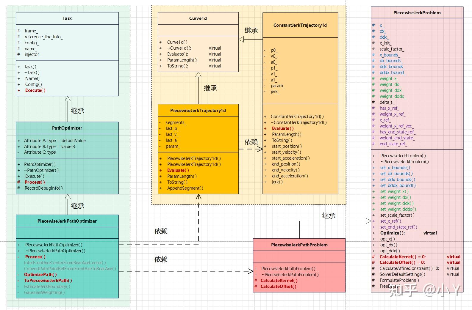
Else
最后附上一张PIECEWISE_JERK_PATH_OPTIMIZER框架图。
参考
[1] Apollo 6.0 QP(二次规划)算法解析
[2] Apollo星火计划学习笔记——Apollo路径规划算法原理与实践
[3] 分段加加速度路径优化
[4] Apollo 6.0的EM Planner (2):路径规划的二次规划QP过程
[5] 【规划】Apollo QSQP接口详解