作为一名数据科学家,我们偶尔会遇到需要对趋势进行建模以预测未来值的情况。虽然人们倾向于关注基于统计或机器学习的算法,但我在这里提出一个不同的选择:卡尔曼滤波器(KF)。
1960 年代初期,Rudolf E. Kalman 彻底改变了使用 KF 建模复杂系统的方式。从引导飞机或航天器到达目的地,到让您的智能手机找到它在这个世界上的位置,该算法融合了数据和数学,以令人难以置信的准确性提供对未来状态的估计。
在本博客中,我们将深入介绍卡尔曼滤波器的工作原理,并展示 Python 中的示例,以强调该技术的真正威力。从一个简单的 2D 示例开始,我们将了解如何修改代码以使其适应更高级的 4D 空间,最后覆盖扩展卡尔曼滤波器(复杂的前身)。和我一起踏上这段旅程,我们将踏上预测算法和过滤器的世界。
卡尔曼滤波器的基础知识
KF 通过构建并持续更新从观察和其他及时测量中收集的一组协方差矩阵(表示噪声和过去状态的统计分布)来提供系统状态的估计。与其他开箱即用的算法不同,可以通过定义系统和外部源之间的数学关系来直接扩展和细化解决方案。虽然这听起来可能相当复杂和错综复杂,但该过程可以概括为两个步骤:预测和更新。这些阶段一起工作,迭代地纠正和完善系统的状态估计。
预测步骤:
此阶段主要是根据模型已知的后验估计和时间步长 Δk 来预测系统的下一个未来状态。在数学上,我们将状态空间的估计表示为:
![]()
其中,F 是我们的状态转换矩阵,它模拟了状态如何从一步演化到另一步,而与控制输入和过程噪声无关。我们的矩阵 B 模拟控制输入 uₖ 对状态的影响。
除了我们对下一个状态的估计之外,该算法还计算由协方差矩阵 P 表示的估计的不确定性:
![]()
预测状态协方差矩阵代表我们预测的置信度和准确性,受系统本身的过程噪声协方差矩阵Q的影响。我们将该矩阵应用于更新步骤中的后续方程,以纠正卡尔曼滤波器在系统上保存的信息,从而改进未来状态估计。
更新步骤:
在更新步骤中,算法对卡尔曼增益、状态估计和协方差矩阵进行更新。卡尔曼增益决定新测量对状态估计的影响有多大。计算包括观测模型矩阵H,它将状态与我们期望接收的测量结果联系起来,以及R测量误差的测量噪声协方差矩阵:
![]()
本质上,K试图平衡预测中的不确定性与测量中存在的不确定性。如上所述,卡尔曼增益用于校正状态估计和协方差,分别由以下方程表示:
![]()
![]()
其中状态估计括号中的计算结果是残差,即实际测量值与模型预测值之间的差异。
卡尔曼滤波器工作原理的真正美妙之处在于其递归本质,在收到新信息时不断更新状态和协方差。这使得模型能够随着时间的推移以统计上最佳的方式进行完善,这对于接收噪声观测流的系统建模来说是特别强大的方法。
卡尔曼滤波器的作用
支持卡尔曼滤波器的方程可能会让您不知所措,并且仅从数学角度充分理解它的工作原理需要了解状态空间(超出了本博客的范围),但我将尝试引入通过一些 Python 示例让它变得生动起来。在最简单的形式中,我们可以将卡尔曼滤波器对象定义为:
import numpy as npclass KalmanFilter:"""An implementation of the classic Kalman Filter for linear dynamic systems.The Kalman Filter is an optimal recursive data processing algorithm whichaims to estimate the state of a system from noisy observations.Attributes:F (np.ndarray): The state transition matrix.B (np.ndarray): The control input marix.H (np.ndarray): The observation matrix.u (np.ndarray): the control input.Q (np.ndarray): The process noise covariance matrix.R (np.ndarray): The measurement noise covariance matrix.x (np.ndarray): The mean state estimate of the previous step (k-1).P (np.ndarray): The state covariance of previous step (k-1)."""def __init__(self, F, B, u, H, Q, R, x0, P0):"""Initializes the Kalman Filter with the necessary matrices and initial state.Parameters:F (np.ndarray): The state transition matrix.B (np.ndarray): The control input marix.H (np.ndarray): The observation matrix.u (np.ndarray): the control input.Q (np.ndarray): The process noise covariance matrix.R (np.ndarray): The measurement noise covariance matrix.x0 (np.ndarray): The initial state estimate.P0 (np.ndarray): The initial state covariance matrix."""self.F = F # State transition matrixself.B = B # Control input matrixself.u = u # Control vectorself.H = H # Observation matrixself.Q = Q # Process noise covarianceself.R = R # Measurement noise covarianceself.x = x0 # Initial state estimateself.P = P0 # Initial estimate covariancedef predict(self):"""Predicts the state and the state covariance for the next time step."""self.x = self.F @ self.x + self.B @ self.uself.P = self.F @ self.P @ self.F.T + self.Qreturn self.xdef update(self, z):"""Updates the state estimate with the latest measurement.Parameters:z (np.ndarray): The measurement at the current step."""y = z - self.H @ self.xS = self.H @ self.P @ self.H.T + self.RK = self.P @ self.H.T @ np.linalg.inv(S)self.x = self.x + K @ yI = np.eye(self.P.shape[0])self.P = (I - K @ self.H) @ self.Preturn self.xChallenges with Non-linear Systems我们将使用predict()和update()函数来迭代前面概述的步骤。上述过滤器设计适用于任何时间序列,为了展示我们的估计与实际情况的比较,让我们构建一个简单的示例:
import numpy as np
import matplotlib.pyplot as plt# Set the random seed for reproducibility
np.random.seed(42)# Simulate the ground truth position of the object
true_velocity = 0.5  # units per time step
num_steps = 50
time_steps = np.linspace(0, num_steps, num_steps)
true_positions = true_velocity * time_steps# Simulate the measurements with noise
measurement_noise = 10  # increase this value to make measurements noisier
noisy_measurements = true_positions + np.random.normal(0, measurement_noise, num_steps)# Plot the true positions and the noisy measurements
plt.figure(figsize=(10, 6))
plt.plot(time_steps, true_positions, label='True Position', color='green')
plt.scatter(time_steps, noisy_measurements, label='Noisy Measurements', color='red', marker='o')plt.xlabel('Time Step')
plt.ylabel('Position')
plt.title('True Position and Noisy Measurements Over Time')
plt.legend()
plt.show()
实际上,“真实位置”是未知的,但我们将在此处绘制它以供参考,“噪声测量”是输入卡尔曼滤波器的观察点。我们将执行矩阵的非常基本的实例化,在某种程度上,这并不重要,因为卡尔曼模型将通过应用卡尔曼增益快速收敛,但在某些情况下对模型执行热启动可能是合理的。
# Kalman Filter Initialization
F = np.array([[1, 1], [0, 1]])   # State transition matrix
B = np.array([[0], [0]])          # No control input
u = np.array([[0]])               # No control input
H = np.array([[1, 0]])            # Measurement function
Q = np.array([[1, 0], [0, 3]])    # Process noise covariance
R = np.array([[measurement_noise**2]]) # Measurement noise covariance
x0 = np.array([[0], [0]])         # Initial state estimate
P0 = np.array([[1, 0], [0, 1]])   # Initial estimate covariancekf = KalmanFilter(F, B, u, H, Q, R, x0, P0)# Allocate space for estimated positions and velocities
estimated_positions = np.zeros(num_steps)
estimated_velocities = np.zeros(num_steps)# Kalman Filter Loop
for t in range(num_steps):# Predictkf.predict()# Updatemeasurement = np.array([[noisy_measurements[t]]])kf.update(measurement)# Store the filtered position and velocityestimated_positions[t] = kf.x[0]estimated_velocities[t] = kf.x[1]# Plot the true positions, noisy measurements, and the Kalman filter estimates
plt.figure(figsize=(10, 6))
plt.plot(time_steps, true_positions, label='True Position', color='green')
plt.scatter(time_steps, noisy_measurements, label='Noisy Measurements', color='red', marker='o')
plt.plot(time_steps, estimated_positions, label='Kalman Filter Estimate', color='blue')plt.xlabel('Time Step')
plt.ylabel('Position')
plt.title('Kalman Filter Estimation Over Time')
plt.legend()
plt.show()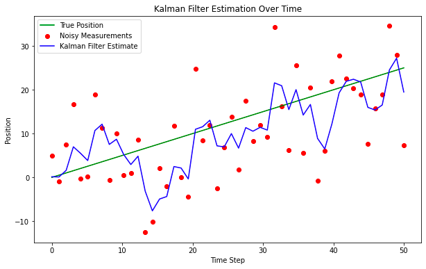
即使采用这种非常简单的解决方案设计,该模型也能很好地穿透噪音找到真实位置。这对于简单的应用程序来说可能没问题,但趋势通常更加微妙,并受到外部事件的影响。为了解决这个问题,我们通常需要修改状态空间表示,还需要修改计算估计值的方式,并在新信息到达时纠正协方差矩阵,让我们用另一个例子来进一步探讨这一点
追踪 4D 移动物体
假设我们想要跟踪物体在空间和时间上的运动,为了使这个例子更加真实,我们将模拟一些作用在物体上的力,从而导致角旋转。为了展示该算法对更高维状态空间表示的适应性,我们将假设线性力,尽管实际上情况并非如此(在此之后我们将探索一个更现实的示例)。下面的代码显示了我们如何针对这种特定场景修改卡尔曼滤波器的示例。
import numpy as np
import matplotlib.pyplot as plt
from mpl_toolkits.mplot3d import Axes3Dclass KalmanFilter:"""An implementation of the classic Kalman Filter for linear dynamic systems.The Kalman Filter is an optimal recursive data processing algorithm whichaims to estimate the state of a system from noisy observations.Attributes:F (np.ndarray): The state transition matrix.B (np.ndarray): The control input marix.H (np.ndarray): The observation matrix.u (np.ndarray): the control input.Q (np.ndarray): The process noise covariance matrix.R (np.ndarray): The measurement noise covariance matrix.x (np.ndarray): The mean state estimate of the previous step (k-1).P (np.ndarray): The state covariance of previous step (k-1)."""def __init__(self, F=None, B=None, u=None, H=None, Q=None, R=None, x0=None, P0=None):"""Initializes the Kalman Filter with the necessary matrices and initial state.Parameters:F (np.ndarray): The state transition matrix.B (np.ndarray): The control input marix.H (np.ndarray): The observation matrix.u (np.ndarray): the control input.Q (np.ndarray): The process noise covariance matrix.R (np.ndarray): The measurement noise covariance matrix.x0 (np.ndarray): The initial state estimate.P0 (np.ndarray): The initial state covariance matrix."""self.F = F  # State transition matrixself.B = B  # Control input matrixself.u = u  # Control inputself.H = H  # Observation matrixself.Q = Q  # Process noise covarianceself.R = R  # Measurement noise covarianceself.x = x0  # Initial state estimateself.P = P0  # Initial estimate covariancedef predict(self):"""Predicts the state and the state covariance for the next time step."""self.x = np.dot(self.F, self.x) + np.dot(self.B, self.u)self.P = np.dot(np.dot(self.F, self.P), self.F.T) + self.Qdef update(self, z):"""Updates the state estimate with the latest measurement.Parameters:z (np.ndarray): The measurement at the current step."""y = z - np.dot(self.H, self.x)S = np.dot(self.H, np.dot(self.P, self.H.T)) + self.RK = np.dot(np.dot(self.P, self.H.T), np.linalg.inv(S))self.x = self.x + np.dot(K, y)self.P = self.P - np.dot(np.dot(K, self.H), self.P)# Parameters for simulation
true_angular_velocity = 0.1  # radians per time step
radius = 20
num_steps = 100
dt = 1  # time step# Create time steps
time_steps = np.arange(0, num_steps*dt, dt)# Ground truth state
true_x_positions = radius * np.cos(true_angular_velocity * time_steps)
true_y_positions = radius * np.sin(true_angular_velocity * time_steps)
true_z_positions = 0.5 * time_steps  # constant velocity in z# Create noisy measurements
measurement_noise = 1.0
noisy_x_measurements = true_x_positions + np.random.normal(0, measurement_noise, num_steps)
noisy_y_measurements = true_y_positions + np.random.normal(0, measurement_noise, num_steps)
noisy_z_measurements = true_z_positions + np.random.normal(0, measurement_noise, num_steps)# Kalman Filter initialization
F = np.array([[1, 0, 0, -radius*dt*np.sin(true_angular_velocity*dt)],[0, 1, 0, radius*dt*np.cos(true_angular_velocity*dt)],[0, 0, 1, 0],[0, 0, 0, 1]])
B = np.zeros((4, 1))
u = np.zeros((1, 1))
H = np.array([[1, 0, 0, 0],[0, 1, 0, 0],[0, 0, 1, 0]])
Q = np.eye(4) * 0.1  # Small process noise
R = measurement_noise**2 * np.eye(3)  # Measurement noise
x0 = np.array([[0], [radius], [0], [true_angular_velocity]])
P0 = np.eye(4) * 1.0kf = KalmanFilter(F, B, u, H, Q, R, x0, P0)# Allocate space for estimated states
estimated_states = np.zeros((num_steps, 4))# Kalman Filter Loop
for t in range(num_steps):# Predictkf.predict()# Updatez = np.array([[noisy_x_measurements[t]],[noisy_y_measurements[t]],[noisy_z_measurements[t]]])kf.update(z)# Store the stateestimated_states[t, :] = kf.x.ravel()# Extract estimated positions
estimated_x_positions = estimated_states[:, 0]
estimated_y_positions = estimated_states[:, 1]
estimated_z_positions = estimated_states[:, 2]# Plotting
fig = plt.figure(figsize=(10, 8))
ax = fig.add_subplot(111, projection='3d')# Plot the true trajectory
ax.plot(true_x_positions, true_y_positions, true_z_positions, label='True Trajectory', color='g')
# Plot the start and end markers for the true trajectory
ax.scatter(true_x_positions[0], true_y_positions[0], true_z_positions[0], label='Start (Actual)', c='green', marker='x', s=100)
ax.scatter(true_x_positions[-1], true_y_positions[-1], true_z_positions[-1], label='End (Actual)', c='red', marker='x', s=100)# Plot the noisy measurements
ax.scatter(noisy_x_measurements, noisy_y_measurements, noisy_z_measurements, label='Noisy Measurements', color='r')# Plot the estimated trajectory
ax.plot(estimated_x_positions, estimated_y_positions, estimated_z_positions, label='Estimated Trajectory', color='b')# Plot settings
ax.set_xlabel('X position')
ax.set_ylabel('Y position')
ax.set_zlabel('Z position')
ax.set_title('3D Trajectory Estimation with Kalman Filter')
ax.legend()plt.show()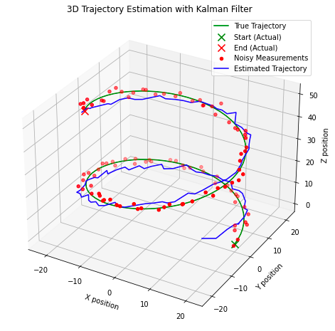
这里需要注意一些有趣的点,在上图中,我们可以看到当我们开始迭代观察结果时,模型如何快速校正到估计的真实状态。该模型在识别系统的真实状态方面也表现得相当好,估计与真实状态(“真实轨迹”)相交。这种设计可能适合某些现实世界的应用,但不适用于作用在系统上的力是非线性的应用。相反,我们需要考虑卡尔曼滤波器的不同应用:扩展卡尔曼滤波器,它是我们迄今为止所探索的线性化输入观测值的非线性的前身。
扩展卡尔曼滤波器
当尝试对系统的观测或动态非线性的系统进行建模时,我们需要应用扩展卡尔曼滤波器(EKF)。该算法与上一个算法的不同之处在于,将雅可比矩阵纳入解中并执行泰勒级数展开以找到状态转移和观测模型的一阶线性近似。为了以数学方式表达这一扩展,我们的关键算法计算现在变为:
![]()
对于状态预测,其中 f 是应用于先前状态估计的非线性状态转换函数,u是先前时间步的控制输入。
![]()
用于误差协方差预测,其中F是状态转换函数相对于P(先前误差协方差)和Q(过程噪声协方差矩阵)的雅可比行列式。
![]()
在时间步k处对测量z的观测,其中h是应用于状态预测的非线性观测函数,具有一些加性观测噪声v。
![]()
我们对卡尔曼增益计算的更新,其中H是相对于状态的观测函数的雅可比行列式,R是测量噪声协方差矩阵。
![]()
状态估计的修改计算结合了卡尔曼增益和非线性观测函数,最后是我们更新误差协方差的方程:
![]()
在最后一个示例中,这将使用 Jocabian 来线性化角旋转对我们对象的非线性影响,并适当修改代码。设计 EKF 比 KF 更具挑战性,因为我们对一阶线性近似的假设可能会无意中将误差引入到我们的状态估计中。此外,雅可比行列式计算可能会变得复杂、计算成本高昂且难以在某些情况下定义,这也可能导致错误。然而,如果设计正确,EKF 通常会优于 KF 实现。
在我们上一个 Python 示例的基础上,我介绍了 EKF 的实现:
import numpy as np
import matplotlib.pyplot as plt
from mpl_toolkits.mplot3d import Axes3Dclass ExtendedKalmanFilter:"""An implementation of the Extended Kalman Filter (EKF).This filter is suitable for systems with non-linear dynamics by linearisingthe system model at each time step using the Jacobian.Attributes:state_transition (callable): The state transition function for the system.jacobian_F (callable): Function to compute the Jacobian of the state transition.H (np.ndarray): The observation matrix.jacobian_H (callable): Function to compute the Jacobian of the observation model.Q (np.ndarray): The process noise covariance matrix.R (np.ndarray): The measurement noise covariance matrix.x (np.ndarray): The initial state estimate.P (np.ndarray): The initial estimate covariance."""def __init__(self, state_transition, jacobian_F, observation_matrix, jacobian_H, Q, R, x, P):"""Constructs the Extended Kalman Filter.Parameters:state_transition (callable): The state transition function.jacobian_F (callable): Function to compute the Jacobian of F.observation_matrix (np.ndarray): Observation matrix.jacobian_H (callable): Function to compute the Jacobian of H.Q (np.ndarray): Process noise covariance.R (np.ndarray): Measurement noise covariance.x (np.ndarray): Initial state estimate.P (np.ndarray): Initial estimate covariance."""self.state_transition = state_transition  # Non-linear state transition functionself.jacobian_F = jacobian_F  # Function to compute Jacobian of Fself.H = observation_matrix  # Observation matrixself.jacobian_H = jacobian_H  # Function to compute Jacobian of Hself.Q = Q  # Process noise covarianceself.R = R  # Measurement noise covarianceself.x = x  # Initial state estimateself.P = P  # Initial estimate covariancedef predict(self, u):"""Predicts the state at the next time step.Parameters:u (np.ndarray): The control input vector."""self.x = self.state_transition(self.x, u)F = self.jacobian_F(self.x, u)self.P = F @ self.P @ F.T + self.Qdef update(self, z):"""Updates the state estimate with a new measurement.Parameters:z (np.ndarray): The measurement vector."""H = self.jacobian_H()y = z - self.H @ self.xS = H @ self.P @ H.T + self.RK = self.P @ H.T @ np.linalg.inv(S)self.x = self.x + K @ yself.P = (np.eye(len(self.x)) - K @ H) @ self.P# Define the non-linear transition and Jacobian functions
def state_transition(x, u):"""Defines the state transition function for the system with non-linear dynamics.Parameters:x (np.ndarray): The current state vector.u (np.ndarray): The control input vector containing time step and rate of change of angular velocity.Returns:np.ndarray: The next state vector as predicted by the state transition function."""dt = u[0]alpha = u[1]x_next = np.array([x[0] - x[3] * x[1] * dt,x[1] + x[3] * x[0] * dt,x[2] + x[3] * dt,x[3],x[4] + alpha * dt])return x_nextdef jacobian_F(x, u):"""Computes the Jacobian matrix of the state transition function.Parameters:x (np.ndarray): The current state vector.u (np.ndarray): The control input vector containing time step and rate of change of angular velocity.Returns:np.ndarray: The Jacobian matrix of the state transition function at the current state."""dt = u[0]# Compute the Jacobian matrix of the state transition functionF = np.array([[1, -x[3]*dt, 0, -x[1]*dt, 0],[x[3]*dt, 1, 0, x[0]*dt, 0],[0, 0, 1, dt, 0],[0, 0, 0, 1, 0],[0, 0, 0, 0, 1]])return Fdef jacobian_H():# Jacobian matrix for the observation function is simply the observation matrixreturn H# Simulation parameters
num_steps = 100
dt = 1.0
alpha = 0.01  # Rate of change of angular velocity# Observation matrix, assuming we can directly observe the x, y, and z position
H = np.eye(3, 5)# Process noise covariance matrix
Q = np.diag([0.1, 0.1, 0.1, 0.1, 0.01])# Measurement noise covariance matrix
R = np.diag([0.5, 0.5, 0.5])# Initial state estimate and covariance
x0 = np.array([0, 20, 0, 0.5, 0.1])  # [x, y, z, v, omega]
P0 = np.eye(5)# Instantiate the EKF
ekf = ExtendedKalmanFilter(state_transition, jacobian_F, H, jacobian_H, Q, R, x0, P0)# Generate true trajectory and measurements
true_states = []
measurements = []
for t in range(num_steps):u = np.array([dt, alpha])true_state = state_transition(x0, u)  # This would be your true system modeltrue_states.append(true_state)measurement = true_state[:3] + np.random.multivariate_normal(np.zeros(3), R)  # Simulate measurement noisemeasurements.append(measurement)x0 = true_state  # Update the true state# Now we run the EKF over the measurements
estimated_states = []
for z in measurements:ekf.predict(u=np.array([dt, alpha]))ekf.update(z=np.array(z))estimated_states.append(ekf.x)# Convert lists to arrays for plotting
true_states = np.array(true_states)
measurements = np.array(measurements)
estimated_states = np.array(estimated_states)# Plotting the results
fig = plt.figure(figsize=(12, 9))
ax = fig.add_subplot(111, projection='3d')# Plot the true trajectory
ax.plot(true_states[:, 0], true_states[:, 1], true_states[:, 2], label='True Trajectory')
# Increase the size of the start and end markers for the true trajectory
ax.scatter(true_states[0, 0], true_states[0, 1], true_states[0, 2], label='Start (Actual)', c='green', marker='x', s=100)
ax.scatter(true_states[-1, 0], true_states[-1, 1], true_states[-1, 2], label='End (Actual)', c='red', marker='x', s=100)# Plot the measurements
ax.scatter(measurements[:, 0], measurements[:, 1], measurements[:, 2], label='Measurements', alpha=0.6)
# Plot the start and end markers for the measurements
ax.scatter(measurements[0, 0], measurements[0, 1], measurements[0, 2], c='green', marker='o', s=100)
ax.scatter(measurements[-1, 0], measurements[-1, 1], measurements[-1, 2], c='red', marker='x', s=100)# Plot the EKF estimate
ax.plot(estimated_states[:, 0], estimated_states[:, 1], estimated_states[:, 2], label='EKF Estimate')ax.set_xlabel('X')
ax.set_ylabel('Y')
ax.set_zlabel('Z')
ax.legend()plt.show()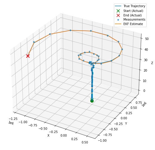
简单总结
在本博客中,我们深入探讨了如何构建和应用卡尔曼滤波器 (KF),以及如何实现扩展卡尔曼滤波器 (EKF)。最后,我们总结一下这些模型的用例、优点和缺点。
KF:该模型适用于线性系统,我们可以假设状态转移和观察矩阵是状态的线性函数(带有一些高斯噪声)。您可以考虑将此算法应用于:
- 跟踪以恒定速度移动的物体的位置和速度
- 如果噪声是随机的或可以用线性模型表示的信号处理应用
- 如果底层关系可以线性建模,则可以进行经济预测
KF 的主要优点是(一旦遵循矩阵计算)该算法非常简单,计算强度比其他方法少,并且可以及时提供系统真实状态的非常准确的预测和估计。缺点是线性假设在复杂的现实场景中通常不成立。
EKF:我们本质上可以将 EKF 视为 KF 的非线性等价物,并得到雅可比行列式的使用支持。如果您正在处理以下问题,您会考虑 EKF:
- 测量和系统动力学通常是非线性的机器人系统
- 通常涉及非恒定速度或角速率变化的跟踪和导航系统,例如跟踪飞机或航天器的跟踪和导航系统。
- 汽车系统在实施最现代“智能”汽车中的巡航控制或车道保持时。
EKF 通常会产生比 KF 更好的估计,特别是对于非线性系统,但由于雅可比矩阵的计算,它的计算量可能会更大。该方法还依赖于泰勒级数展开式的一阶线性近似,这对于高度非线性系统可能不是合适的假设。添加雅可比行列式还可能使模型的设计更具挑战性,因此尽管有其优点,但为了简单性和互操作性而实现 KF 可能更合适。