目录
一、前言
二、神经网络架构
三、算法实现
1、导入包
2、实现类
3、训练函数
4、权重参数矩阵初始化
5、参数矩阵变换向量
6、向量变换权重参数矩阵
7、进行梯度下降
7.1、损失函数
7.1.1、前向传播
7.2、反向传播
8、预测函数
四、完整代码
五、手写数字识别
一、前言
读者需要了解神经网络的基础知识,可以参考神经网络(深度学习,计算机视觉,得分函数,损失函数,前向传播,反向传播,激活函数)
本文为大家详细的描述了,实现神经网络的逻辑,代码。并且用手写识别来实验,结果基本实现了神经网络的要求。
二、神经网络架构

想一想:
1.输入数据:特征值(手写数字识别是像素点,784个特征)
2.W1,W2,W3矩阵的形状
3.前向传播
4.激活函数(用Sigmoid)
5.反向传播
6.偏置项
7.损失()
8.得出W1,W2,W3对损失有多大影响,公式如下:
算法流程(简便版):
三、算法实现
1、导入包
import  numpy as np
from Neural_Network_Lab.utils.features import prepare_for_training
from Neural_Network_Lab.utils.hypothesis import sigmoid,sigmoid_gradient
这里utils包用来封装数据预处理,和Sigmoid函数
数据预处理:
import numpy as np
from .normalize import normalizedef generate_polynomials(dataset, polynomial_degree, normalize_data=False):"""变换方法:x1, x2, x1^2, x2^2, x1*x2, x1*x2^2, etc."""features_split = np.array_split(dataset, 2, axis=1)dataset_1 = features_split[0]dataset_2 = features_split[1](num_examples_1, num_features_1) = dataset_1.shape(num_examples_2, num_features_2) = dataset_2.shapeif num_examples_1 != num_examples_2:raise ValueError('Can not generate polynomials for two sets with different number of rows')if num_features_1 == 0 and num_features_2 == 0:raise ValueError('Can not generate polynomials for two sets with no columns')if num_features_1 == 0:dataset_1 = dataset_2elif num_features_2 == 0:dataset_2 = dataset_1num_features = num_features_1 if num_features_1 < num_examples_2 else num_features_2dataset_1 = dataset_1[:, :num_features]dataset_2 = dataset_2[:, :num_features]polynomials = np.empty((num_examples_1, 0))for i in range(1, polynomial_degree + 1):for j in range(i + 1):polynomial_feature = (dataset_1 ** (i - j)) * (dataset_2 ** j)polynomials = np.concatenate((polynomials, polynomial_feature), axis=1)if normalize_data:polynomials = normalize(polynomials)[0]return polynomials
Sigmoid函数:
import numpy as npdef sigmoid(matrix):"""Applies sigmoid function to NumPy matrix"""return 1 / (1 + np.exp(-matrix))2、实现类
多层感知机 初始化:数据,标签,网络层次(用列表表示如三层[784,25,10]表示输入层784个神经元,25个隐藏层神经元,10个输出层神经元),数据是否标准化处理。
class MultilayerPerceptron:def __init__(self,data,labels,layers,normalize_data=False):data_processed = prepare_for_training(data,normalize_data=normalize_data)[0]self.data = data_processedself.labels = labelsself.layers = layers # [ 784 ,25 ,10]self.normalize_data = normalize_dataself.thetas = MultilayerPerceptron.thetas_init(layers)
3、训练函数
输入迭代次数,学习率,进行梯度下降算法,更新权重参数矩阵,得到最终的权重参数矩阵,和损失值。矩阵不好进行更新操作,可以把它拉成向量。
def train(self,max_ietrations = 1000,alpha = 0.1):#方便矩阵更新 拉长 把矩阵拉成向量unrolled_theta = MultilayerPerceptron.thetas_unroll(self.thetas)(optimized_theta, cost_history) = MultilayerPerceptron.gradient_descent(self.data,self.labels,unrolled_theta,self.layers,max_ietrations,alpha)self.thetas = MultilayerPerceptron.thetas_roll(optimized_theta,self.layers)return self.thetas,cost_history4、权重参数矩阵初始化
根据网络层次可以确定,矩阵的大小,用字典存储。
@staticmethoddef thetas_init(layers):num_layers = len(layers)thetas = {} #用字典形式 key:表示第几层 vlues:权重参数矩阵for layer_index in range(num_layers-1):'''会执行两次: 得到两组参数矩阵 25 * 785 , 10 * 26'''in_count = layers[layer_index]out_count = layers[layer_index+1]#初始化 初始值小#这里需要考虑偏置项,偏置的个数与输出的个数一样thetas[layer_index]=np.random.rand(out_count,in_count+1) * 0.05 #加一列输入特征return thetas5、参数矩阵变换向量
将权重参数矩阵变换成向量
@staticmethoddef thetas_unroll(thetas):#拼接成一个向量num_theta_layers = len(thetas)unrolled_theta = np.array([])for theta_layer_index in range(num_theta_layers):unrolled_theta = np.hstack((unrolled_theta,thetas[theta_layer_index].flatten()))return unrolled_theta6、向量变换权重参数矩阵
后边前向传播时需要进行矩阵乘法,需要变换回来
@staticmethoddef thetas_roll(unrolled_theta,layers):num_layers = len(layers)thetas = {}unrolled_shift = 0for layer_index in range(num_layers - 1):in_count = layers[layer_index]out_count = layers[layer_index + 1]thetas_width = in_count + 1thetas_height = out_countthetas_volume = thetas_width * thetas_heightstart_index = unrolled_shiftend_index =unrolled_shift + thetas_volumelayer_theta_unrolled = unrolled_theta[start_index:end_index]thetas[layer_index] = layer_theta_unrolled.reshape((thetas_height,thetas_width))unrolled_shift = unrolled_shift + thetas_volumereturn thetas7、进行梯度下降
1. 损失函数,计算损失值
2. 计算梯度值
3. 更新参数
那么得先要实现损失函数,计算损失值。
7.1、损失函数
实现损失函数,得到损失值得要实现前向传播走一次
7.1.1、前向传播
@staticmethoddef feedforword_propagation(data,thetas,layers):num_layers = len(layers)num_examples = data.shape[0]in_layer_activation = data #输入层#逐层计算 隐藏层for layer_index in range(num_layers - 1):theta = thetas[layer_index]out_layer_activation = sigmoid(np.dot(in_layer_activation,theta.T)) #输出层# 正常计算之后是num_examples * 25 ,但是要考虑偏置项 变成num_examples * 26out_layer_activation = np.hstack((np.ones((num_examples,1)),out_layer_activation))in_layer_activation = out_layer_activation#返回输出层结果,不要偏置项return in_layer_activation[:,1:]损失函数:
@staticmethoddef cost_function(data,labels,thetas,layers):num_layers = len(layers)num_examples = data.shape[0]num_labels = layers[-1]#前向传播走一次predictions = MultilayerPerceptron.feedforword_propagation(data,thetas,layers)#制作标签,每一个样本的标签都是one-dotbitwise_labels = np.zeros((num_examples,num_labels))for example_index in range(num_examples):bitwise_labels[example_index][labels[example_index][0]] = 1#咱们的预测值是概率值y= 7 [0,0,0,0,0,0,1,0,0,0] 在正确值的位置上概率越大越好 在错误值的位置上概率越小越好bit_set_cost = np.sum(np.log(predictions[bitwise_labels == 1]))bit_not_set_cost = np.sum(np.log(1 - predictions[bitwise_labels == 0]))cost = (-1/num_examples) * (bit_set_cost+bit_not_set_cost)return cost7.2、反向传播
在梯度下降的过程中,要实现参数矩阵的更新,必须要实现反向传播。利用上述的公式,进行运算即可得到。
@staticmethoddef back_propagation(data,labels,thetas,layers):num_layers = len(layers)(num_examples,num_features) = data.shapenum_label_types = layers[-1]deltas = {} # 算出每一层对结果的影响#初始化for layer_index in range(num_layers - 1):in_count = layers[layer_index]out_count = layers[layer_index + 1]deltas[layer_index] = np.zeros((out_count,in_count+1)) #25 * 785 10 *26for example_index in range(num_examples):layers_inputs = {}layers_activations = {}layers_activation = data[example_index,:].reshape((num_features,1))layers_activations[0] = layers_activation#逐层计算for layer_index in range(num_layers - 1):layer_theta = thetas[layer_index] #得到当前的权重参数值 : 25 *785 10 *26layer_input = np.dot(layer_theta,layers_activation) # 第一次 得到 25 * 1 第二次: 10 * 1layers_activation = np.vstack((np.array([[1]]),sigmoid(layer_input))) #完成激活函数,加上一个偏置参数layers_inputs[layer_index+1] = layer_input # 后一层计算结果layers_activations[layer_index +1] = layers_activation # 后一层完成激活的结果output_layer_activation = layers_activation[1:,:]#计算输出层和结果的差异delta = {}#标签处理bitwise_label = np.zeros((num_label_types,1))bitwise_label[labels[example_index][0]] = 1#计算输出结果和真实值之间的差异delta[num_layers-1] = output_layer_activation - bitwise_label #输出层#遍历 L,L-1,L-2...2for layer_index in range(num_layers - 2,0,-1):layer_theta = thetas[layer_index]next_delta = delta[layer_index+1]layer_input = layers_inputs[layer_index]layer_input = np.vstack((np.array((1)),layer_input))#按照公式计算delta[layer_index] = np.dot(layer_theta.T,next_delta)*sigmoid(layer_input)#过滤掉偏置参数delta[layer_index] = delta[layer_index][1:,:]#计算梯度值for layer_index in range(num_layers-1):layer_delta = np.dot(delta[layer_index+1],layers_activations[layer_index].T) #微调矩阵deltas[layer_index] = deltas[layer_index] + layer_delta #第一次25 * 785 第二次 10 * 26for layer_index in range(num_layers-1):deltas[layer_index] = deltas[layer_index] * (1/num_examples) #公式return deltas实现一次梯度下降:
@staticmethoddef gradient_step(data,labels,optimized_theta,layers):theta = MultilayerPerceptron.thetas_roll(optimized_theta,layers)#反向传播BPthetas_rolled_gradinets = MultilayerPerceptron.back_propagation(data,labels,theta,layers)thetas_unrolled_gradinets = MultilayerPerceptron.thetas_unroll(thetas_rolled_gradinets)return thetas_unrolled_gradinets实现梯度下降:
@staticmethoddef gradient_descent(data,labels,unrolled_theta,layers,max_ietrations,alpha):#1. 计算损失值#2. 计算梯度值#3. 更新参数optimized_theta = unrolled_theta #最好的theta值cost_history = [] #损失值的记录for i in range(max_ietrations):if i % 10 == 0 :print("当前迭代次数:",i)cost = MultilayerPerceptron.cost_function(data,labels,MultilayerPerceptron.thetas_roll(optimized_theta,layers),layers)cost_history.append(cost)theta_gradient = MultilayerPerceptron.gradient_step(data,labels,optimized_theta,layers)optimized_theta = optimized_theta - alpha * theta_gradientreturn optimized_theta,cost_history8、预测函数
输入测试数据,前向传播走一次,得到预测值
def predict(self,data):data_processed = prepare_for_training(data,normalize_data = self.normalize_data)[0]num_examples = data_processed.shape[0]predictions = MultilayerPerceptron.feedforword_propagation(data_processed,self.thetas,self.layers)return np.argmax(predictions,axis=1).reshape((num_examples,1))四、完整代码
import  numpy as np
from Neural_Network_Lab.utils.features import prepare_for_training
from Neural_Network_Lab.utils.hypothesis import sigmoid,sigmoid_gradientclass MultilayerPerceptron:def __init__(self,data,labels,layers,normalize_data=False):data_processed = prepare_for_training(data,normalize_data=normalize_data)[0]self.data = data_processedself.labels = labelsself.layers = layers #  [  784 ,25 ,10]self.normalize_data = normalize_dataself.thetas = MultilayerPerceptron.thetas_init(layers)def predict(self,data):data_processed = prepare_for_training(data,normalize_data = self.normalize_data)[0]num_examples = data_processed.shape[0]predictions = MultilayerPerceptron.feedforword_propagation(data_processed,self.thetas,self.layers)return np.argmax(predictions,axis=1).reshape((num_examples,1))def train(self,max_ietrations = 1000,alpha = 0.1):#方便矩阵更新 拉长  把矩阵拉成向量unrolled_theta = MultilayerPerceptron.thetas_unroll(self.thetas)(optimized_theta, cost_history) = MultilayerPerceptron.gradient_descent(self.data,self.labels,unrolled_theta,self.layers,max_ietrations,alpha)self.thetas = MultilayerPerceptron.thetas_roll(optimized_theta,self.layers)return self.thetas,cost_history@staticmethoddef gradient_descent(data,labels,unrolled_theta,layers,max_ietrations,alpha):#1. 计算损失值#2. 计算梯度值#3. 更新参数optimized_theta = unrolled_theta #最好的theta值cost_history = []  #损失值的记录for i in range(max_ietrations):if i % 10 == 0 :print("当前迭代次数:",i)cost  = MultilayerPerceptron.cost_function(data,labels,MultilayerPerceptron.thetas_roll(optimized_theta,layers),layers)cost_history.append(cost)theta_gradient = MultilayerPerceptron.gradient_step(data,labels,optimized_theta,layers)optimized_theta = optimized_theta - alpha * theta_gradientreturn optimized_theta,cost_history@staticmethoddef gradient_step(data,labels,optimized_theta,layers):theta = MultilayerPerceptron.thetas_roll(optimized_theta,layers)#反向传播BPthetas_rolled_gradinets = MultilayerPerceptron.back_propagation(data,labels,theta,layers)thetas_unrolled_gradinets = MultilayerPerceptron.thetas_unroll(thetas_rolled_gradinets)return thetas_unrolled_gradinets@staticmethoddef back_propagation(data,labels,thetas,layers):num_layers = len(layers)(num_examples,num_features) = data.shapenum_label_types = layers[-1]deltas = {} # 算出每一层对结果的影响#初始化for layer_index in  range(num_layers - 1):in_count = layers[layer_index]out_count = layers[layer_index + 1]deltas[layer_index] = np.zeros((out_count,in_count+1)) #25 * 785 10 *26for example_index in range(num_examples):layers_inputs = {}layers_activations = {}layers_activation = data[example_index,:].reshape((num_features,1))layers_activations[0] = layers_activation#逐层计算for layer_index in range(num_layers - 1):layer_theta = thetas[layer_index]  #得到当前的权重参数值 : 25 *785 10 *26layer_input = np.dot(layer_theta,layers_activation) # 第一次 得到 25 * 1 第二次: 10 * 1layers_activation = np.vstack((np.array([[1]]),sigmoid(layer_input))) #完成激活函数,加上一个偏置参数layers_inputs[layer_index+1] = layer_input # 后一层计算结果layers_activations[layer_index +1] = layers_activation # 后一层完成激活的结果output_layer_activation = layers_activation[1:,:]#计算输出层和结果的差异delta = {}#标签处理bitwise_label = np.zeros((num_label_types,1))bitwise_label[labels[example_index][0]] = 1#计算输出结果和真实值之间的差异delta[num_layers-1] = output_layer_activation - bitwise_label #输出层#遍历 L,L-1,L-2...2for layer_index in range(num_layers - 2,0,-1):layer_theta = thetas[layer_index]next_delta = delta[layer_index+1]layer_input = layers_inputs[layer_index]layer_input = np.vstack((np.array((1)),layer_input))#按照公式计算delta[layer_index] = np.dot(layer_theta.T,next_delta)*sigmoid(layer_input)#过滤掉偏置参数delta[layer_index] = delta[layer_index][1:,:]#计算梯度值for layer_index in  range(num_layers-1):layer_delta = np.dot(delta[layer_index+1],layers_activations[layer_index].T)  #微调矩阵deltas[layer_index] = deltas[layer_index] + layer_delta #第一次25 * 785 第二次 10 * 26for layer_index in range(num_layers-1):deltas[layer_index] = deltas[layer_index] * (1/num_examples)return deltas@staticmethoddef cost_function(data,labels,thetas,layers):num_layers = len(layers)num_examples = data.shape[0]num_labels = layers[-1]#前向传播走一次predictions = MultilayerPerceptron.feedforword_propagation(data,thetas,layers)#制作标签,每一个样本的标签都是one-dotbitwise_labels = np.zeros((num_examples,num_labels))for example_index in range(num_examples):bitwise_labels[example_index][labels[example_index][0]] = 1#咱们的预测值是概率值y= 7 [0,0,0,0,0,0,1,0,0,0]    在正确值的位置上概率越大越好 在错误值的位置上概率越小越好bit_set_cost = np.sum(np.log(predictions[bitwise_labels == 1]))bit_not_set_cost = np.sum(np.log(1 - predictions[bitwise_labels == 0]))cost = (-1/num_examples) * (bit_set_cost+bit_not_set_cost)return cost@staticmethoddef feedforword_propagation(data,thetas,layers):num_layers = len(layers)num_examples = data.shape[0]in_layer_activation = data #输入层#逐层计算 隐藏层for layer_index in range(num_layers - 1):theta = thetas[layer_index]out_layer_activation = sigmoid(np.dot(in_layer_activation,theta.T)) #输出层# 正常计算之后是num_examples * 25 ,但是要考虑偏置项 变成num_examples * 26out_layer_activation = np.hstack((np.ones((num_examples,1)),out_layer_activation))in_layer_activation = out_layer_activation#返回输出层结果,不要偏置项return in_layer_activation[:,1:]@staticmethoddef thetas_roll(unrolled_theta,layers):num_layers = len(layers)thetas = {}unrolled_shift = 0for layer_index in range(num_layers - 1):in_count = layers[layer_index]out_count = layers[layer_index + 1]thetas_width = in_count + 1thetas_height = out_countthetas_volume = thetas_width * thetas_heightstart_index = unrolled_shiftend_index =unrolled_shift + thetas_volumelayer_theta_unrolled = unrolled_theta[start_index:end_index]thetas[layer_index] = layer_theta_unrolled.reshape((thetas_height,thetas_width))unrolled_shift = unrolled_shift + thetas_volumereturn thetas@staticmethoddef thetas_unroll(thetas):#拼接成一个向量num_theta_layers = len(thetas)unrolled_theta = np.array([])for theta_layer_index in range(num_theta_layers):unrolled_theta = np.hstack((unrolled_theta,thetas[theta_layer_index].flatten()))return unrolled_theta@staticmethoddef thetas_init(layers):num_layers = len(layers)thetas = {} #用字典形式 key:表示第几层 vlues:权重参数矩阵for layer_index in range(num_layers-1):'''会执行两次: 得到两组参数矩阵 25 * 785 , 10 * 26'''in_count = layers[layer_index]out_count = layers[layer_index+1]#初始化 初始值小#这里需要考虑偏置项,偏置的个数与输出的个数一样thetas[layer_index]=np.random.rand(out_count,in_count+1) * 0.05 #加一列输入特征return thetas
五、手写数字识别
数据集(读者可以找找下载,我就不放链接了>_<): 


共一万个样本,第一列为标签值,一列表示像素点的值共28*28共784个像素点。
import numpy as np
import pandas as pd
import matplotlib.pyplot as plt
import matplotlib.image as mping
import math
from Neural_Network_Lab.Multilayer_Perceptron import MultilayerPerceptrondata = pd.read_csv('../Neural_Network_Lab/data/mnist-demo.csv')
#展示数据
numbers_to_display = 25
num_cells = math.ceil(math.sqrt(numbers_to_display))
plt.figure(figsize=(10,10))
for plot_index in range(numbers_to_display):digit = data[plot_index:plot_index+1].valuesdigit_label = digit[0][0]digit_pixels = digit[0][1:]image_size = int(math.sqrt(digit_pixels.shape[0]))frame = digit_pixels.reshape((image_size,image_size))plt.subplot(num_cells,num_cells,plot_index+1)plt.imshow(frame,cmap = 'Greys')plt.title(digit_label)
plt.subplots_adjust(wspace=0.5,hspace=0.5)
plt.show()train_data = data.sample(frac= 0.8)
test_data = data.drop(train_data.index)train_data = train_data.values
test_data = test_data.valuesnum_training_examples = 8000X_train = train_data[:num_training_examples,1:]
y_train = train_data[:num_training_examples,[0]]X_test = test_data[:,1:]
y_test = test_data[:,[0]]layers = [784,25,10]
normalize_data = True
max_iteration = 500
alpha = 0.1multilayerperceptron = MultilayerPerceptron(X_train,y_train,layers,normalize_data)
(thetas,cost_history) = multilayerperceptron.train(max_iteration,alpha)
plt.plot(range(len(cost_history)),cost_history)
plt.xlabel('Grident steps')
plt.ylabel('cost')
plt.show()y_train_predictions = multilayerperceptron.predict(X_train)
y_test_predictions = multilayerperceptron.predict(X_test)train_p = np.sum((y_train_predictions == y_train) / y_train.shape[0] * 100)
test_p = np.sum((y_test_predictions == y_test) / y_test.shape[0] * 100)print("训练集准确率:",train_p)
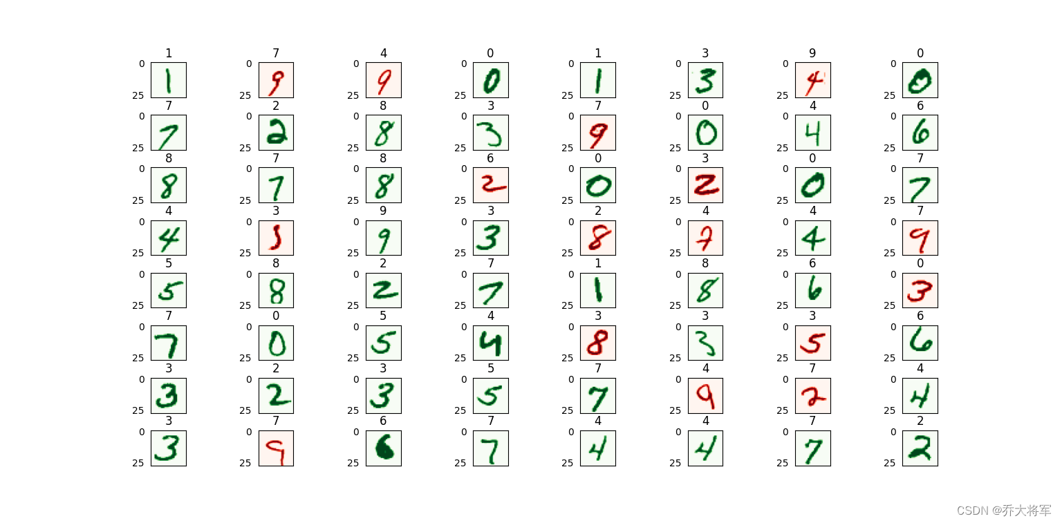
print("测试集准确率:",test_p)numbers_to_display = 64
num_cells = math.ceil(math.sqrt(numbers_to_display))
plt.figure(figsize=(15,15))
for plot_index in range(numbers_to_display):digit_label = y_test[plot_index,0]digit_pixels = X_test[plot_index,:]predicted_label = y_test_predictions[plot_index][0]image_size = int(math.sqrt(digit_pixels.shape[0]))frame = digit_pixels.reshape((image_size,image_size))plt.subplot(num_cells,num_cells,plot_index+1)color_map = 'Greens' if predicted_label == digit_label else 'Reds'plt.imshow(frame,cmap = color_map)plt.title(predicted_label)plt.tick_params(axis='both',which='both',bottom=False,left=False,labelbottom=False)plt.subplots_adjust(wspace=0.5,hspace=0.5)
plt.show()训练集8000个,测试集2000个,迭代次数500次


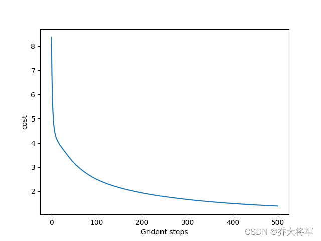
这里准确率不高,读者可以自行调整参数,改变迭代次数,网络层次都可以哦。