前言
系列专栏:【深度学习:算法项目实战】✨︎
涉及医疗健康、财经金融、商业零售、食品饮料、运动健身、交通运输、环境科学、社交媒体以及文本和图像处理等诸多领域,讨论了各种复杂的深度神经网络思想,如卷积神经网络、循环神经网络、生成对抗网络、门控循环单元、长短期记忆、自然语言处理、深度强化学习、大型语言模型和迁移学习。
本章将使用 Tensorflow 进行情感分析,以阐述文本分类!在需要捕捉序列信息时,循环神经网络(RNN)就能派上用场(另一种应用可能包括时间序列、下一个单词预测等)。由于其内部记忆因素,它能记住过去的序列和当前的输入,这使它能够捕捉上下文而不仅仅是单个单词。
目录
- 1. 相关数据集
- 1.1 导入必要库
- 1.2 加载数据集
- 2. 构建RNN模型
- 2.1 SimpleRNN (also called Vanilla RNN)
- 2.2 Gated Recurrent Units (GRU)
- 2.3 Long Short Term Memory (LSTM)
- 2.4 Bi-directional LSTM Model
- 3. 模型评估
- 3.1 绘制GRU训练和验证的accuracy曲线
- 3.2 绘制GRU训练和验证损失的Loss曲线
- 4. 结论
1. 相关数据集
1.1 导入必要库
import numpy as np
import pandas as pd
import seaborn as sns
import matplotlib.pyplot as pltfrom tensorflow.keras.models import Sequential
from tensorflow.keras.datasets import imdb
from tensorflow.keras.layers import Input, SimpleRNN, LSTM, GRU, Bidirectional, Dense, Embedding
1.2 加载数据集
我们将使用 Keras IMDB 数据集。词汇量大小是一个参数,用于获取包含整个文本数据语料库中出现次数最多的单词的数据。
①获取数据集
获取在整个评论文本数据语料库中出现次数最多的 5000 个评论词语
# Getting reviews with words that come under 5000 most occurring words in the entire corpus of textual review data
vocab_size = 5000
(x_train, y_train), (x_test, y_test) = imdb.load_data(num_words=vocab_size)print(x_train[0])
[1, 14, 22, 16, 43, 530, 973, 1622, 1385, 65, 458, 4468, 66, 3941, 4, 173, 36, 256, 5, 25, 100, 43, 838, 112, 50, 670, 2, 9, 35, 480, 284, 5, 150, 4, 172, 112, 167, 2, 336, 385, 39, 4, 172, 4536, 1111, 17, 546, 38, 13, 447, 4, 192, 50, 16, 6, 147, 2025, 19, 14, 22, 4, 1920, 4613, 469, 4, 22, 71, 87, 12, 16, 43, 530, 38, 76, 15, 13, 1247, 4, 22, 17, 515, 17, 12, 16, 626, 18, 2, 5, 62, 386, 12, 8, 316, 8, 106, 5, 4, 2223, 2, 16, 480, 66, 3785, 33, 4, 130, 12, 16, 38, 619, 5, 25, 124, 51, 36, 135, 48, 25, 1415, 33, 6, 22, 12, 215, 28, 77, 52, 5, 14, 407, 16, 82, 2, 8, 4, 107, 117, 2, 15, 256, 4, 2, 7, 3766, 5, 723, 36, 71, 43, 530, 476, 26, 400, 317, 46, 7, 4, 2, 1029, 13, 104, 88, 4, 381, 15, 297, 98, 32, 2071, 56, 26, 141, 6, 194, 2, 18, 4, 226, 22, 21, 134, 476, 26, 480, 5, 144, 30, 2, 18, 51, 36, 28, 224, 92, 25, 104, 4, 226, 65, 16, 38, 1334, 88, 12, 16, 283, 5, 16, 4472, 113, 103, 32, 15, 16, 2, 19, 178, 32]
这些数字是索引值,于此我们可以看到任何评论
# Getting all the words from word_index dictionary
word_idx = imdb.get_word_index()# Originally the index number of a value and not a key,
# hence converting the index as key and the words as values
word_idx = {i: word for word, i in word_idx.items()}# again printing the review
print([word_idx[i] for i in x_train[0]])
['the', 'as', 'you', 'with', 'out', 'themselves', 'powerful', 'lets', 'loves', 'their', 'becomes', 'reaching', 'had', 'journalist', 'of', 'lot', 'from', 'anyone', 'to', 'have', 'after', 'out', 'atmosphere', 'never', 'more', 'room', 'and', 'it', 'so', 'heart', 'shows', 'to', 'years', 'of', 'every', 'never', 'going', 'and', 'help', 'moments', 'or', 'of', 'every', 'chest', 'visual', 'movie', 'except', 'her', 'was', 'several', 'of', 'enough', 'more', 'with', 'is', 'now', 'current', 'film', 'as', 'you', 'of', 'mine', 'potentially', 'unfortunately', 'of', 'you', 'than', 'him', 'that', 'with', 'out', 'themselves', 'her', 'get', 'for', 'was', 'camp', 'of', 'you', 'movie', 'sometimes', 'movie', 'that', 'with', 'scary', 'but', 'and', 'to', 'story', 'wonderful', 'that', 'in', 'seeing', 'in', 'character', 'to', 'of', '70s', 'and', 'with', 'heart', 'had', 'shadows', 'they', 'of', 'here', 'that', 'with', 'her', 'serious', 'to', 'have', 'does', 'when', 'from', 'why', 'what', 'have', 'critics', 'they', 'is', 'you', 'that', "isn't", 'one', 'will', 'very', 'to', 'as', 'itself', 'with', 'other', 'and', 'in', 'of', 'seen', 'over', 'and', 'for', 'anyone', 'of', 'and', 'br', "show's", 'to', 'whether', 'from', 'than', 'out', 'themselves', 'history', 'he', 'name', 'half', 'some', 'br', 'of', 'and', 'odd', 'was', 'two', 'most', 'of', 'mean', 'for', '1', 'any', 'an', 'boat', 'she', 'he', 'should', 'is', 'thought', 'and', 'but', 'of', 'script', 'you', 'not', 'while', 'history', 'he', 'heart', 'to', 'real', 'at', 'and', 'but', 'when', 'from', 'one', 'bit', 'then', 'have', 'two', 'of', 'script', 'their', 'with', 'her', 'nobody', 'most', 'that', 'with', "wasn't", 'to', 'with', 'armed', 'acting', 'watch', 'an', 'for', 'with', 'and', 'film', 'want', 'an']
让我们检查一下这个数据集中的评论范围。
# Get the minimum and the maximum length of reviews
print("Max length of a review:", len(max((x_train+x_test), key=len)))
print("Min length of a review:", len(min((x_train+x_test), key=len)))
Max length of a review: 2697
Min length of a review: 70
我们可以看到,最长的评论有 2697 个字,最短的只有 70 个字。在使用神经网络时,重要的是使所有输入都有固定的大小。为了实现这一目标,我们将对评论句子进行填充。
from tensorflow.keras.preprocessing import sequence# Keeping a fixed length of all reviews to max 400 words
max_words = 400x_train = sequence.pad_sequences(x_train, maxlen=max_words)
x_test = sequence.pad_sequences(x_test, maxlen=max_words)x_valid, y_valid = x_train[:64], y_train[:64]
x_train_, y_train_ = x_train[64:], y_train[64:]
2. 构建RNN模型
2.1 SimpleRNN (also called Vanilla RNN)
它们是递归神经网络的最基本形式,试图记忆顺序信息。然而,它们也存在爆炸梯度和消失梯度的问题。
# fixing every word's embedding size to be 32
embd_len = 32# Creating a RNN model
RNN_model = Sequential(name="Simple_RNN")
RNN_model.add(Input(shape=(max_words,)))
RNN_model.add(Embedding(vocab_size,embd_len))# In case of a stacked(more than one layer of RNN)
# use return_sequences=True
RNN_model.add(SimpleRNN(128,activation='tanh',return_sequences=False))
RNN_model.add(Dense(1, activation='sigmoid'))# printing model summary
print(RNN_model.summary())# Compiling model
RNN_model.compile(loss="binary_crossentropy",optimizer='adam',metrics=['accuracy']
)# Training the model
history = RNN_model.fit(x_train_, y_train_,batch_size=64,epochs=5,verbose=1,validation_data=(x_valid, y_valid))# Printing model score on test data
print()
print("Simple_RNN Score---> ", RNN_model.evaluate(x_test, y_test, verbose=0))
Model: "Simple_RNN"
┏━━━━━━━━━━━━━━━━━━━━━━━━━━━━━━━━━━━━━━┳━━━━━━━━━━━━━━━━━━━━━━━━━━━━━┳━━━━━━━━━━━━━━━━━┓
┃ Layer (type)                         ┃ Output Shape                ┃         Param # ┃
┡━━━━━━━━━━━━━━━━━━━━━━━━━━━━━━━━━━━━━━╇━━━━━━━━━━━━━━━━━━━━━━━━━━━━━╇━━━━━━━━━━━━━━━━━┩
│ embedding (Embedding)                │ (None, 400, 32)             │         160,000 │
├──────────────────────────────────────┼─────────────────────────────┼─────────────────┤
│ simple_rnn (SimpleRNN)               │ (None, 128)                 │          20,608 │
├──────────────────────────────────────┼─────────────────────────────┼─────────────────┤
│ dense (Dense)                        │ (None, 1)                   │             129 │
└──────────────────────────────────────┴─────────────────────────────┴─────────────────┘Total params: 180,737 (706.00 KB)Trainable params: 180,737 (706.00 KB)Non-trainable params: 0 (0.00 B)
None
Epoch 1/5
390/390 ━━━━━━━━━━━━━━━━━━━━ 29s 70ms/step - accuracy: 0.5083 - loss: 0.7005 - val_accuracy: 0.4219 - val_loss: 0.7201
Epoch 2/5
390/390 ━━━━━━━━━━━━━━━━━━━━ 27s 69ms/step - accuracy: 0.6551 - loss: 0.6139 - val_accuracy: 0.7344 - val_loss: 0.5395
Epoch 3/5
390/390 ━━━━━━━━━━━━━━━━━━━━ 27s 69ms/step - accuracy: 0.7021 - loss: 0.5714 - val_accuracy: 0.6875 - val_loss: 0.6699
Epoch 4/5
390/390 ━━━━━━━━━━━━━━━━━━━━ 27s 68ms/step - accuracy: 0.7384 - loss: 0.5209 - val_accuracy: 0.6719 - val_loss: 0.6933
Epoch 5/5
390/390 ━━━━━━━━━━━━━━━━━━━━ 27s 68ms/step - accuracy: 0.7895 - loss: 0.4497 - val_accuracy: 0.6094 - val_loss: 0.7292Simple_RNN Score--->  [0.6092072129249573, 0.6787999868392944]
简单 RNN 的测试准确率为 67.87%。简单 RNN 的局限性在于,由于梯度消失问题,它无法很好地处理长句子。
2.2 Gated Recurrent Units (GRU)
GRU 是一种鲜为人知但同样强大的算法,可解决简单 RNN 的局限性。
# Defining GRU model
gru_model = Sequential(name="GRU_Model")
gru_model.add(Input(shape=(max_words,)))
gru_model.add(Embedding(vocab_size,embd_len))
gru_model.add(GRU(128,activation='tanh',return_sequences=False))
gru_model.add(Dense(1, activation='sigmoid'))# Printing the Summary
print(gru_model.summary())# Compiling the model
gru_model.compile(loss="binary_crossentropy",optimizer='adam',metrics=['accuracy']
)# Training the GRU model
history2 = gru_model.fit(x_train_, y_train_,batch_size=64,epochs=5,verbose=1,validation_data=(x_valid, y_valid))# Printing model score on test data
print()
print("GRU model Score---> ", gru_model.evaluate(x_test, y_test, verbose=0))
Model: "GRU_Model"
┏━━━━━━━━━━━━━━━━━━━━━━━━━━━━━━━━━━━━━━┳━━━━━━━━━━━━━━━━━━━━━━━━━━━━━┳━━━━━━━━━━━━━━━━━┓
┃ Layer (type)                         ┃ Output Shape                ┃         Param # ┃
┡━━━━━━━━━━━━━━━━━━━━━━━━━━━━━━━━━━━━━━╇━━━━━━━━━━━━━━━━━━━━━━━━━━━━━╇━━━━━━━━━━━━━━━━━┩
│ embedding_1 (Embedding)              │ (None, 400, 32)             │         160,000 │
├──────────────────────────────────────┼─────────────────────────────┼─────────────────┤
│ gru (GRU)                            │ (None, 128)                 │          62,208 │
├──────────────────────────────────────┼─────────────────────────────┼─────────────────┤
│ dense_1 (Dense)                      │ (None, 1)                   │             129 │
└──────────────────────────────────────┴─────────────────────────────┴─────────────────┘Total params: 222,337 (868.50 KB)Trainable params: 222,337 (868.50 KB)Non-trainable params: 0 (0.00 B)
None
Epoch 1/5
390/390 ━━━━━━━━━━━━━━━━━━━━ 138s 351ms/step - accuracy: 0.6241 - loss: 0.6236 - val_accuracy: 0.8750 - val_loss: 0.3197
Epoch 2/5
390/390 ━━━━━━━━━━━━━━━━━━━━ 138s 353ms/step - accuracy: 0.8513 - loss: 0.3522 - val_accuracy: 0.8750 - val_loss: 0.2863
Epoch 3/5
390/390 ━━━━━━━━━━━━━━━━━━━━ 142s 363ms/step - accuracy: 0.8958 - loss: 0.2657 - val_accuracy: 0.9062 - val_loss: 0.2370
Epoch 4/5
390/390 ━━━━━━━━━━━━━━━━━━━━ 140s 360ms/step - accuracy: 0.9208 - loss: 0.2083 - val_accuracy: 0.8906 - val_loss: 0.2334
Epoch 5/5
390/390 ━━━━━━━━━━━━━━━━━━━━ 141s 362ms/step - accuracy: 0.9425 - loss: 0.1643 - val_accuracy: 0.9062 - val_loss: 0.2388GRU model Score--->  [0.298039048910141, 0.883840024471283]
GRU 的测试准确率为 88.38%。GRU 是 RNN 的一种形式,由于其训练参数相对较少,因此比简单的 RNN 更好,通常也比 LSTM 更快。
2.3 Long Short Term Memory (LSTM)
与简单的 RNN 相比,LSTM 能更好地捕捉顺序信息的记忆。要了解 LSTM 的理论方面,请访问文章 Long Short Term Memory Networks Explanation。由于 LSTM 比 GRU 更加复杂,因此训练速度较慢,但总的来说,LSTM 比 GRU 具有更高的准确性。
# Defining LSTM model
lstm_model = Sequential(name="LSTM_Model")
lstm_model.add(Input(shape=(max_words,)))
lstm_model.add(Embedding(vocab_size,embd_len))
lstm_model.add(LSTM(128,activation='relu',return_sequences=False))
lstm_model.add(Dense(1, activation='sigmoid'))# Printing Model Summary
print(lstm_model.summary())# Compiling the model
lstm_model.compile(loss="binary_crossentropy",optimizer='adam',metrics=['accuracy']
)# Training the model
history3 = lstm_model.fit(x_train_, y_train_,batch_size=64,epochs=5,verbose=2,validation_data=(x_valid, y_valid))# Displaying the model accuracy on test data
print()
print("LSTM model Score---> ", lstm_model.evaluate(x_test, y_test, verbose=0))
Model: "LSTM_Model"
┏━━━━━━━━━━━━━━━━━━━━━━━━━━━━━━━━━━━━━━┳━━━━━━━━━━━━━━━━━━━━━━━━━━━━━┳━━━━━━━━━━━━━━━━━┓
┃ Layer (type)                         ┃ Output Shape                ┃         Param # ┃
┡━━━━━━━━━━━━━━━━━━━━━━━━━━━━━━━━━━━━━━╇━━━━━━━━━━━━━━━━━━━━━━━━━━━━━╇━━━━━━━━━━━━━━━━━┩
│ embedding_2 (Embedding)              │ (None, 400, 32)             │         160,000 │
├──────────────────────────────────────┼─────────────────────────────┼─────────────────┤
│ lstm (LSTM)                          │ (None, 128)                 │          82,432 │
├──────────────────────────────────────┼─────────────────────────────┼─────────────────┤
│ dense_2 (Dense)                      │ (None, 1)                   │             129 │
└──────────────────────────────────────┴─────────────────────────────┴─────────────────┘Total params: 242,561 (947.50 KB)Trainable params: 242,561 (947.50 KB)Non-trainable params: 0 (0.00 B)
None
Epoch 1/5
390/390 ━━━━━━━━━━━━━━━━━━━━ 111s 280ms/step - accuracy: 0.5024 - loss: 6.9317e-06 - val_accuracy: 0.4375 - val_loss: 6.9350e-06
Epoch 2/5
390/390 ━━━━━━━━━━━━━━━━━━━━ 110s 283ms/step - accuracy: 0.5067 - loss: 6.9304e-06 - val_accuracy: 0.5625 - val_loss: 6.9288e-06
Epoch 3/5
390/390 ━━━━━━━━━━━━━━━━━━━━ 109s 279ms/step - accuracy: 0.5345 - loss: 6.9282e-06 - val_accuracy: 0.4062 - val_loss: 6.9411e-06
Epoch 4/5
390/390 ━━━━━━━━━━━━━━━━━━━━ 108s 278ms/step - accuracy: 0.5178 - loss: 6.9252e-06 - val_accuracy: 0.6562 - val_loss: 6.9168e-06
Epoch 5/5
390/390 ━━━━━━━━━━━━━━━━━━━━ 108s 278ms/step - accuracy: 0.5456 - loss: 6.9193e-06 - val_accuracy: 0.6250 - val_loss: 6.8995e-06LSTM model Score--->  [6.911340278747957e-06, 0.5701599717140198]
LSTM 模型的测试准确率为 57.02%。
2.4 Bi-directional LSTM Model
双向 LSTMS 是传统 LSTMS 的衍生。在这里,两个 LSTM 被用来捕捉输入的前向和后向序列。这有助于比普通 LSTM 更好地捕捉上下文。
# Defining Bidirectional LSTM model
bi_lstm_model = Sequential(name="Bidirectional_LSTM")
bi_lstm_model.add(Input(shape=(max_words,)))
bi_lstm_model.add(Embedding(vocab_size,embd_len))
bi_lstm_model.add(Bidirectional(LSTM(128,activation='tanh',return_sequences=False)))
bi_lstm_model.add(Dense(1, activation='sigmoid'))# Printing model summary
print(bi_lstm_model.summary())# Compiling model summary
bi_lstm_model.compile(
loss="binary_crossentropy",
optimizer='adam',
metrics=['accuracy']
)# Training the model
history4 = bi_lstm_model.fit(x_train_, y_train_,batch_size=64,epochs=5,validation_data=(x_test, y_test))# Printing model score on test data
print()
print("Bidirectional LSTM model Score---> ",bi_lstm_model.evaluate(x_test, y_test, verbose=0))
Model: "Bidirectional_LSTM"
┏━━━━━━━━━━━━━━━━━━━━━━━━━━━━━━━━━━━━━━┳━━━━━━━━━━━━━━━━━━━━━━━━━━━━━┳━━━━━━━━━━━━━━━━━┓
┃ Layer (type)                         ┃ Output Shape                ┃         Param # ┃
┡━━━━━━━━━━━━━━━━━━━━━━━━━━━━━━━━━━━━━━╇━━━━━━━━━━━━━━━━━━━━━━━━━━━━━╇━━━━━━━━━━━━━━━━━┩
│ embedding_3 (Embedding)              │ (None, 400, 32)             │         160,000 │
├──────────────────────────────────────┼─────────────────────────────┼─────────────────┤
│ bidirectional (Bidirectional)        │ (None, 256)                 │         164,864 │
├──────────────────────────────────────┼─────────────────────────────┼─────────────────┤
│ dense_3 (Dense)                      │ (None, 1)                   │             257 │
└──────────────────────────────────────┴─────────────────────────────┴─────────────────┘Total params: 325,121 (1.24 MB)Trainable params: 325,121 (1.24 MB)Non-trainable params: 0 (0.00 B)
None
Epoch 1/5
390/390 ━━━━━━━━━━━━━━━━━━━━ 262s 667ms/step - accuracy: 0.6694 - loss: 0.5770 - val_accuracy: 0.8386 - val_loss: 0.3661
Epoch 2/5
390/390 ━━━━━━━━━━━━━━━━━━━━ 273s 700ms/step - accuracy: 0.8530 - loss: 0.3601 - val_accuracy: 0.8574 - val_loss: 0.3379
Epoch 3/5
390/390 ━━━━━━━━━━━━━━━━━━━━ 280s 717ms/step - accuracy: 0.8906 - loss: 0.2807 - val_accuracy: 0.8515 - val_loss: 0.3501
Epoch 4/5
390/390 ━━━━━━━━━━━━━━━━━━━━ 283s 726ms/step - accuracy: 0.9031 - loss: 0.2486 - val_accuracy: 0.8701 - val_loss: 0.3361
Epoch 5/5
390/390 ━━━━━━━━━━━━━━━━━━━━ 284s 729ms/step - accuracy: 0.9215 - loss: 0.2038 - val_accuracy: 0.8676 - val_loss: 0.3228Bidirectional LSTM model Score--->  [0.32283490896224976, 0.8676400184631348]
双向 LSTM 的测试得分率为 86.76%。
3. 模型评估
在所有模型中,对于给定的 IMDB 评论数据集,GRU 模型的准确率最高。
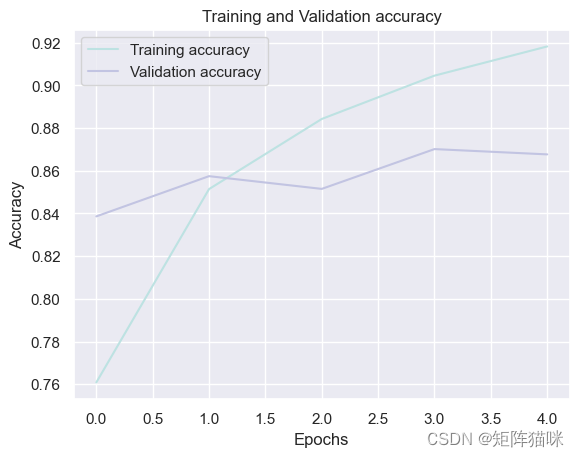
3.1 绘制GRU训练和验证的accuracy曲线
sns.set_theme()
history_df = pd.DataFrame(history2.history)plt.plot(history_df.loc[:, ['accuracy']], "#BDE2E2", label='Training accuracy')
plt.plot(history_df.loc[:, ['val_accuracy']], "#C2C4E2", label='Validation accuracy')plt.title('Training and Validation accuracy')
plt.xlabel('Epochs')
plt.ylabel('Accuracy')
plt.legend()
plt.show()
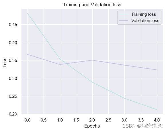
3.2 绘制GRU训练和验证损失的Loss曲线
history_df = pd.DataFrame(history2.history)plt.plot(history_df.loc[:, ['loss']], "#BDE2E2", label='Training loss')
plt.plot(history_df.loc[:, ['val_loss']],"#C2C4E2", label='Validation loss')
plt.title('Training and Validation loss')
plt.xlabel('Epochs')
plt.ylabel('Loss')
plt.legend(loc="best")plt.show()
4. 结论
我们以基本形式测试了递归神经网络的所有主要类型,在所有上述模型中,层数、激活函数、批量大小和历时等所有常用超参数均保持不变。从 SimpleRNN 到双向 LSTM,随着可训练参数数量的增加,模型的复杂性也在增加。 在所有模型中,对于给定的 IMDB 评论数据集,GRU 模型的准确率最高。