【大模型】基于Hugging Face调用及微调大模型（1）

文章目录

一、前言
二、Transformer
三、Hugging Face
- 3.1 Hugging Face Dataset
- 3. 2 Hugging Face Tokenizer
- 3.3 Hugging Face Transformer
- 3.4 Hugging Face Accelerate
四、基于Hugging Face调用模型
- 4.1 调用示例
- 4.2 调用流程概述
- - 4.2.1 Tokenizer
  - 4.2.2 模型的加载
  - 4.2.3 模型基本逻辑
  - 4.2.4 加入输出头
参考资料

一、前言

ChatGPT的基本原理以及预训练大语言模型的发展史，我们知道ChatGPT和所有预训练大语言模型的核心是什么？其实就是 Transformer，Hugging Face 的火爆离不开他们开源的这个 Transformers 库。这个开源库里有数万个我们可以直接调用的模型。很多场景下，这个开源模型已经足够我们使用了。接下来我们就从Transformer的架构和具体的案例来介绍Hugging Face Transformer。

二、Transformer

Transformer 是一种用于自然语言处理和其它序列到序列任务的神经网络模型，它是在2017年由Vaswani等人提出来的，Transformer的核心模块是通过自注意力机制（Self Attention）捕捉序列之间的依赖关系。

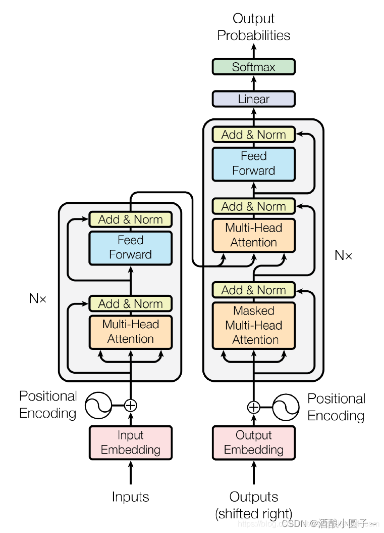
我们在之前的博客中介绍过Transformer，具体参考：Transformer 模型详解

三、Hugging Face

Hugging Face Transformers 是一家公司，在Hugging Face提供的API中，我们几乎可以下载到所有前面提到的预训练大模型的全部信息和各种参数。我们可以认为这些模型在Hugging Face基本就是开源的了，我们只需要拿过来微调或者重新训练这些模型。

用官方的话来说，Hugging Face Transformers 是一个用于自然语言处理的Python库，提供了预训练的语言模型和工具，使得研究者和工程师能够轻松的训练使用共享最先进的NLP模型，其中包括BERT、GPT、RoBERTa、XLNet、DistillBERT等等。

通过 Transformers 可以轻松的用这些预训练模型进行文本分类、命名实体识别、机器翻译、问答系统等NLP任务。这个库还提供了方便的API、示例代码和文档，让我们使用这些模型或者学习模型变得非常简单。

Hugging Face官网：https://huggingface.co/
在这里插入图片描述

Hugging Face的主要产品包括Hugging Face Dataset、Hugging Face Tokenizer、Hugging Face Transformer和Hugging Face Accelerate。

Hugging Face Dataset：是一个库，用于轻松访问和共享音频、计算机视觉和自然语言处理（NLP）任务的数据集。只需一行代码即可加载数据集，并使用强大的数据处理方法快速准备好数据集，以便在深度学习模型中进行训练。在Apache Arrow格式的支持下，以零拷贝读取处理大型数据集，没有任何内存限制，以实现最佳速度和效率。
Hugging Face Tokenizer：是一个用于将文本转换为数字表示形式的库。它支持多种编码器，包括BERT、GPT-2等，并提供了一些高级对齐方法，可以用于映射原始字符串（字符和单词）和标记空间之间的关系。
Hugging Face Transformer：是一个用于自然语言处理（NLP）任务的库。它提供了各种预训练模型，包括BERT、GPT-2等，并提供了一些高级功能，例如控制生成文本的长度、温度等。
Hugging Face Accelerate：是一个用于加速训练和推理的库。它支持各种硬件加速器，例如GPU、TPU等，并提供了一些高级功能，例如混合精度训练、梯度累积等。

3.1 Hugging Face Dataset

Hugging Face Dataset是一个公共数据集仓库，用于轻松访问和共享音频、计算机视觉和自然语言处理（NLP）任务的数据集。只需一行代码即可加载数据集，并使用强大的数据处理方法快速准备好数据集，以便在深度学习模型中进行训练。

在Apache Arrow格式的支持下，以零拷贝读取处理大型数据集，没有任何内存限制，以实现最佳速度和效率。Hugging Face Dataset还与拥抱面部中心深度集成，使您可以轻松加载数据集并与更广泛的机器学习社区共享数据集。

在花时间下载数据集之前，快速获取有关数据集的一些常规信息通常会很有帮助。数据集的信息存储在 DatasetInfo 中，可以包含数据集描述、要素和数据集大小等信息。

使用 load_dataset_builder（）函数加载数据集构建器并检查数据集的属性，而无需提交下载：

>>> from datasets import load_dataset_builder
>>> ds_builder = load_dataset_builder("rotten_tomatoes")# Inspect dataset description
>>> ds_builder.info.description
Movie Review Dataset. This is a dataset of containing 5,331 positive and 5,331 negative processed sentences from Rotten Tomatoes movie reviews. This data was first used in Bo Pang and Lillian Lee, ``Seeing stars: Exploiting class relationships for sentiment categorization with respect to rating scales.'', Proceedings of the ACL, 2005.# Inspect dataset features
>>> ds_builder.info.features
{'label': ClassLabel(num_classes=2, names=['neg', 'pos'], id=None),'text': Value(dtype='string', id=None)}

如果您对数据集感到满意，请使用 load_dataset（）加载它：

from datasets import load_datasetdataset = load_dataset("rotten_tomatoes", split="train")

3. 2 Hugging Face Tokenizer

Tokenizers 提供了当今最常用的分词器的实现，重点是性能和多功能性。这些分词器也用于Transformers。

Tokenizer 把文本序列输入到模型之前的预处理，相当于数据预处理的环节，因为模型是不可能直接读文字信息的，还是需要经过分词处理，把文本变成一个个token，每个模型比如BERT、GPT需要的Tokenizer都不一样，它们都有自己的字典，因为每一个模型它的训练语料库是不一样的，所以它的token和它的字典大小、token的格式都会各有不同。整体来讲，就是给各种各样的词进行分词，然后编码，以123456来代表词的状态，这个就是Tokenizer的作用。

所以，Tokenizer的任务就是把输入的文本转换成一个一个的标记，它还可以负责对文本序列的清洗、截断、填充进行处理。简而言之，就是为了满足具体模型所要求的格式。

主要特点：

使用当今最常用的分词器训练新的词汇表并进行标记化。
由于Rust实现，因此非常快速（训练和标记化），在服务器CPU上对1GB文本进行标记化不到20秒。
易于使用，但也非常多功能。
旨在用于研究和生产。
完全对齐跟踪。即使进行破坏性规范化，也始终可以获得与任何令牌对应的原始句子部分。
执行所有预处理：截断、填充、添加模型所需的特殊令牌。

这里演示如何使用 BPE 模型实例化一个：classTokenizer

from tokenizers import Tokenizer
from tokenizers.models import BPE
tokenizer = Tokenizer(BPE(unk_token="[UNK]"))

3.3 Hugging Face Transformer

Transformers提供API和工具，可轻松下载和训练最先进的预训练模型。使用预训练模型可以降低计算成本、碳足迹，并节省训练模型所需的时间和资源。这些模型支持不同模态中的常见任务，例如：

自然语言处理：文本分类、命名实体识别、问答、语言建模、摘要、翻译、多项选择和文本生成。
计算机视觉：图像分类、目标检测和分割。
音频：自动语音识别和音频分类。
多模式：表格问答、光学字符识别、从扫描文档中提取信息、视频分类和视觉问答。

Transformers支持PyTorch、TensorFlow和JAX之间的框架互操作性。这提供了在模型的每个阶段使用不同框架的灵活性；在一个框架中用三行代码训练一个模型，在另一个框架中加载它进行推理。模型还可以导出到ONNX和TorchScript等格式，以在生产环境中部署。

# 导入必要的库
from transformers import AutoModelForSequenceClassification# 初始化分词器和模型
model_name = "bert-base-cased"
model = AutoModelForSequenceClassification.from_pretrained(model_name, num_labels=2)# 将文本编码为模型期望的张量格式
inputs = tokenizer(dataset["train"]["text"][:10], padding=True, truncation=True, return_tensors="pt")# 将编码后的张量输入模型进行预测
outputs = model(**inputs)# 获取预测结果和标签
predictions = outputs.logits.argmax(dim=-1)

3.4 Hugging Face Accelerate

Accelerate 是一个库，只需添加四行代码，即可在任何分布式配置中运行相同的 PyTorch 代码！简而言之，大规模的训练和推理变得简单、高效和适应性强。

from accelerate import Acceleratoraccelerator = Accelerator()model, optimizer, training_dataloader, scheduler = accelerator.prepare(model, optimizer, training_dataloader, scheduler
)

四、基于Hugging Face调用模型

首先需要安装Hugging Face必要的库：

pip install transformers

4.1 调用示例

首先安装 transformers 依赖包：

pip install transformers


from transformers import pipeline#用人家设计好的流程完成一些简单的任务
classifier = pipeline("sentiment-analysis")
classifier(["I've been waiting for a HuggingFace course my whole life.","I hate this so much!",]
)

这里重点讲讲pipeline，它是hugging face的基本工具，可以理解为一个端到端(end-to-end)的一键调用Transformer模型的工具。它具备了数据预处理、模型处理、模型输出后处理等步骤，可以直接输入原始数据，然后给出预测结果，十分方便，在第三部分调用流程中再详细说明。通过pipeline，可以很方便地调用预训练模型！

符合预期的正常结果，输出情感分类的结果：

[{'label': 'POSITIVE', 'score': 0.9598049521446228},{'label': 'NEGATIVE', 'score': 0.9994558691978455}]

不符合预期的异常结果，输出报错信息：

OSError: We couldn't connect to 'https://huggingface.co' to load this file, couldn't find it in the cached files and it looks like google/mt5-small is not the path to a directory containing a file named config.json. Checkout your internet connection or see how to run the library in offline mode at 'https://huggingface.co/docs/transformers/installation#offline-mode'.

【报错原因】：Hugging Face模型在国外，国内服务器无法访问到国外的模型，需要将模型下载到本地来加载。

【解决步骤】：
在HuggingFace官方找到对应的model：
在这里插入图片描述
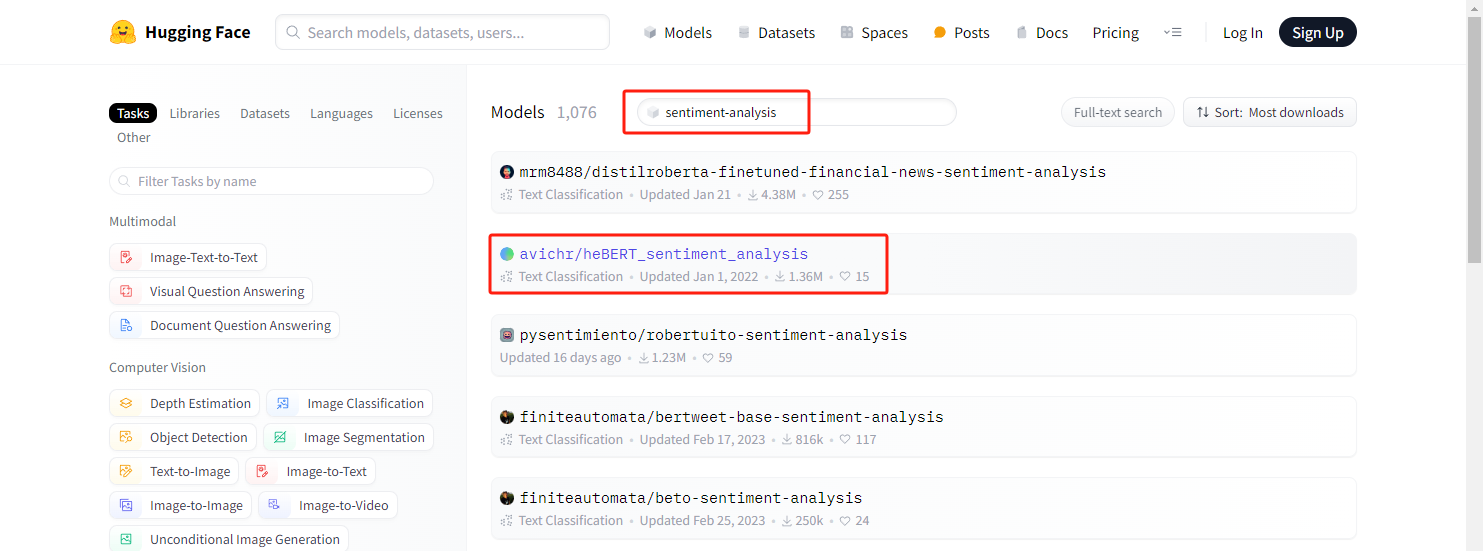
可以看到有非常多 sentiment-analysis 相关的模型，这里我们下载 avichr/heBERT_sentiment_analysis 这个model的相关文件：

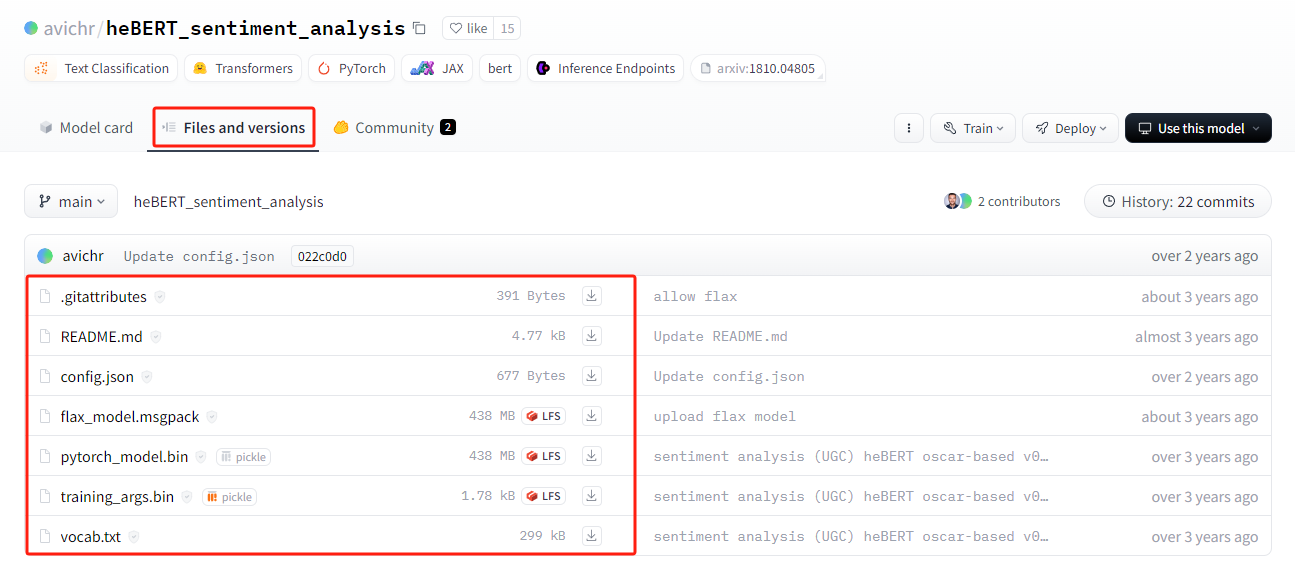
将下载的文件放到本地"./models/sentiment_analysis" 目录下，并将代码修改为：

from transformers import pipeline
model_path = "./models/sentiment_analysis"
classifier = pipeline("sentiment-analysis", model=model_path)  # 通过本地路径加载模型
classifier(["I've been waiting for a HuggingFace course my whole life.","I hate this so much!",]
)

4.2 调用流程概述

首先原始文本用Tokenizer进行分词处理得到输入的文本，然后通过模型进行学习，学习之后进行处理、预测分析。huggingface有个好处，分词器、数据集、模型都封装好了！很方便。
在这里插入图片描述

4.2.1 Tokenizer

Tokenizer会做3件事：

分词，分字以及特殊字符（起始，终止，间隔，分类等特殊字符可以自己设计的）
对每一个token映射得到一个ID（每个词都会对应一个唯一的ID）
还有一些辅助信息也可以得到，比如当前词属于哪个句子（还有一些MASK，表示是否是原来的词还是特殊字符等）

Hugging Face中自带AutoTokenizer工具，可以自动根据模型来判断采用哪个分词器：

from transformers import AutoTokenizer#自动判断checkpoint = "distilbert-base-uncased-finetuned-sst-2-english"#根据这个模型所对应的来加载
tokenizer = AutoTokenizer.from_pretrained(checkpoint)

输入文本：

raw_inputs = ["I've been waiting for a this course my whole life.","I hate this so much!",
]
inputs = tokenizer(raw_inputs, padding=True, truncation=True, return_tensors="pt")
print(inputs)

打印结果（得到两个字典映射，‘input_ids’，一个tensor集合，每个词所对应的ID集合；attention_mask，一个tensor集合，表示是否是原来的词还是特殊字符等）：

{'input_ids': tensor([[ 101, 1045, 1005, 2310, 2042, 3403, 2005, 1037, 2023, 2607, 2026, 2878,2166, 1012,  102],[ 101, 1045, 5223, 2023, 2061, 2172,  999,  102,    0,    0,    0,    0,0,    0,    0]]), 'attention_mask': tensor([[1, 1, 1, 1, 1, 1, 1, 1, 1, 1, 1, 1, 1, 1, 1],[1, 1, 1, 1, 1, 1, 1, 1, 0, 0, 0, 0, 0, 0, 0]])}

如果想根据id重新获得原始句子，如下操作：

tokenizer.decode([ 101, 1045, 1005, 2310, 2042, 3403, 2005, 1037, 2023, 2607, 2026, 2878,2166, 1012,  102])

生成的文本会存在特殊字符，这些特殊字符是因为人家模型训练的时候就加入了这个东西，所以这里默认也加入了（google系的处理）

"[CLS] i've been waiting for a this course my whole life. [SEP]"

4.2.2 模型的加载

模型的加载直接指定好名字即可（先不加输出层），这里checkpoint相当于一个文本，只是方便引用，checkpoint在hugging face中也是专门用来保留原来模型，然后再来训练的。

另外AutoModel类也做下说明，AutoModel类及其相关模型类覆盖了非常多模型。它能够根据checkpoint名称分析得到合适的模型架构，并且使用该架构实例化model，方便后续调用。

from transformers import AutoModelcheckpoint = "distilbert-base-uncased-finetuned-sst-2-english"
model = AutoModel.from_pretrained(checkpoint)
model

打印出来模型架构，就是DistilBertModel（蒸馏后的bert模型，模型参数大约只有原来的60%，训练更快，但准确率下降不多）的架构了，能看到embeddings层、transformer层，看得还比较清晰：

DistilBertModel((embeddings): Embeddings((word_embeddings): Embedding(30522, 768, padding_idx=0)(position_embeddings): Embedding(512, 768)(LayerNorm): LayerNorm((768,), eps=1e-12, elementwise_affine=True)(dropout): Dropout(p=0.1, inplace=False))(transformer): Transformer((layer): ModuleList((0): TransformerBlock((attention): MultiHeadSelfAttention((dropout): Dropout(p=0.1, inplace=False)(q_lin): Linear(in_features=768, out_features=768, bias=True)(k_lin): Linear(in_features=768, out_features=768, bias=True)(v_lin): Linear(in_features=768, out_features=768, bias=True)(out_lin): Linear(in_features=768, out_features=768, bias=True))(sa_layer_norm): LayerNorm((768,), eps=1e-12, elementwise_affine=True)(ffn): FFN((dropout): Dropout(p=0.1, inplace=False)(lin1): Linear(in_features=768, out_features=3072, bias=True)(lin2): Linear(in_features=3072, out_features=768, bias=True))(output_layer_norm): LayerNorm((768,), eps=1e-12, elementwise_affine=True))(1): TransformerBlock((attention): MultiHeadSelfAttention((dropout): Dropout(p=0.1, inplace=False)(q_lin): Linear(in_features=768, out_features=768, bias=True)(k_lin): Linear(in_features=768, out_features=768, bias=True)(v_lin): Linear(in_features=768, out_features=768, bias=True)(out_lin): Linear(in_features=768, out_features=768, bias=True))(sa_layer_norm): LayerNorm((768,), eps=1e-12, elementwise_affine=True)(ffn): FFN((dropout): Dropout(p=0.1, inplace=False)(lin1): Linear(in_features=768, out_features=3072, bias=True)(lin2): Linear(in_features=3072, out_features=768, bias=True))(output_layer_norm): LayerNorm((768,), eps=1e-12, elementwise_affine=True))(2): TransformerBlock((attention): MultiHeadSelfAttention((dropout): Dropout(p=0.1, inplace=False)(q_lin): Linear(in_features=768, out_features=768, bias=True)(k_lin): Linear(in_features=768, out_features=768, bias=True)(v_lin): Linear(in_features=768, out_features=768, bias=True)(out_lin): Linear(in_features=768, out_features=768, bias=True))(sa_layer_norm): LayerNorm((768,), eps=1e-12, elementwise_affine=True)(ffn): FFN((dropout): Dropout(p=0.1, inplace=False)(lin1): Linear(in_features=768, out_features=3072, bias=True)(lin2): Linear(in_features=3072, out_features=768, bias=True))(output_layer_norm): LayerNorm((768,), eps=1e-12, elementwise_affine=True))(3): TransformerBlock((attention): MultiHeadSelfAttention((dropout): Dropout(p=0.1, inplace=False)(q_lin): Linear(in_features=768, out_features=768, bias=True)(k_lin): Linear(in_features=768, out_features=768, bias=True)(v_lin): Linear(in_features=768, out_features=768, bias=True)(out_lin): Linear(in_features=768, out_features=768, bias=True))(sa_layer_norm): LayerNorm((768,), eps=1e-12, elementwise_affine=True)(ffn): FFN((dropout): Dropout(p=0.1, inplace=False)(lin1): Linear(in_features=768, out_features=3072, bias=True)(lin2): Linear(in_features=3072, out_features=768, bias=True))(output_layer_norm): LayerNorm((768,), eps=1e-12, elementwise_affine=True))(4): TransformerBlock((attention): MultiHeadSelfAttention((dropout): Dropout(p=0.1, inplace=False)(q_lin): Linear(in_features=768, out_features=768, bias=True)(k_lin): Linear(in_features=768, out_features=768, bias=True)(v_lin): Linear(in_features=768, out_features=768, bias=True)(out_lin): Linear(in_features=768, out_features=768, bias=True))(sa_layer_norm): LayerNorm((768,), eps=1e-12, elementwise_affine=True)(ffn): FFN((dropout): Dropout(p=0.1, inplace=False)(lin1): Linear(in_features=768, out_features=3072, bias=True)(lin2): Linear(in_features=3072, out_features=768, bias=True))(output_layer_norm): LayerNorm((768,), eps=1e-12, elementwise_affine=True))(5): TransformerBlock((attention): MultiHeadSelfAttention((dropout): Dropout(p=0.1, inplace=False)(q_lin): Linear(in_features=768, out_features=768, bias=True)(k_lin): Linear(in_features=768, out_features=768, bias=True)(v_lin): Linear(in_features=768, out_features=768, bias=True)(out_lin): Linear(in_features=768, out_features=768, bias=True))(sa_layer_norm): LayerNorm((768,), eps=1e-12, elementwise_affine=True)(ffn): FFN((dropout): Dropout(p=0.1, inplace=False)(lin1): Linear(in_features=768, out_features=3072, bias=True)(lin2): Linear(in_features=3072, out_features=768, bias=True))(output_layer_norm): LayerNorm((768,), eps=1e-12, elementwise_affine=True))))
)

从里面取一个TransformerBlock进行分析，如下所示，可以看出由 注意力层+标准化层+前馈神经网络（全连接）层+标准化层 组成，可以看到每一层的逻辑，然后由多个TransformerBlock堆叠。哈哈，有这个东东要想改某一层只需要动动手调一调就行了！

TransformerBlock((attention): MultiHeadSelfAttention((dropout): Dropout(p=0.1, inplace=False)(q_lin): Linear(in_features=768, out_features=768, bias=True)(k_lin): Linear(in_features=768, out_features=768, bias=True)(v_lin): Linear(in_features=768, out_features=768, bias=True)(out_lin): Linear(in_features=768, out_features=768, bias=True))(sa_layer_norm): LayerNorm((768,), eps=1e-12, elementwise_affine=True)(ffn): FFN((dropout): Dropout(p=0.1, inplace=False)(lin1): Linear(in_features=768, out_features=3072, bias=True)(lin2): Linear(in_features=3072, out_features=768, bias=True))(output_layer_norm): LayerNorm((768,), eps=1e-12, elementwise_affine=True))

看下输出层的结构，这里**表示分配字典，按照参数顺序依次赋值：

outputs = model(**inputs)
print(outputs.last_hidden_state.shape)

输出：

torch.Size([2, 15, 768])

4.2.3 模型基本逻辑

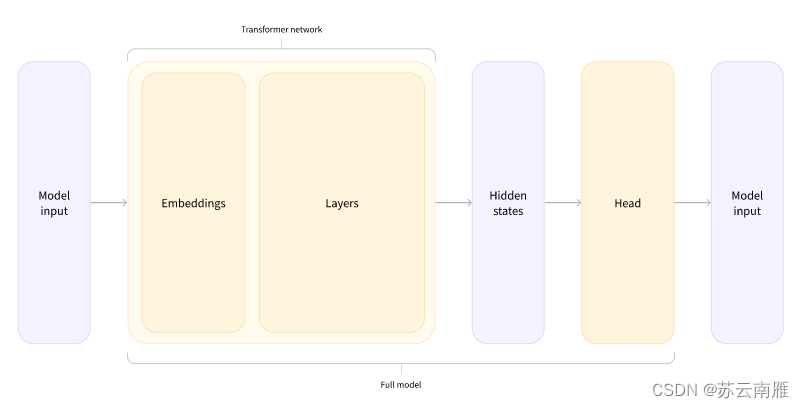
根据上面代码总结模型的逻辑：input—>词嵌入—>Transformer—>隐藏层—>Head层。

在这里插入图片描述

4.2.4 加入输出头

from transformers import AutoModelForSequenceClassificationcheckpoint = "distilbert-base-uncased-finetuned-sst-2-english"
model = AutoModelForSequenceClassification.from_pretrained(checkpoint)
outputs = model(**inputs)
print(outputs.logits.shape)

这里就得到分类后的结果：

torch.Size([2, 2])

再来看看模型的结构：

model

输出：

DistilBertForSequenceClassification((distilbert): DistilBertModel((embeddings): Embeddings((word_embeddings): Embedding(30522, 768, padding_idx=0)(position_embeddings): Embedding(512, 768)(LayerNorm): LayerNorm((768,), eps=1e-12, elementwise_affine=True)(dropout): Dropout(p=0.1, inplace=False))(transformer): Transformer((layer): ModuleList((0): TransformerBlock((attention): MultiHeadSelfAttention((dropout): Dropout(p=0.1, inplace=False)(q_lin): Linear(in_features=768, out_features=768, bias=True)(k_lin): Linear(in_features=768, out_features=768, bias=True)(v_lin): Linear(in_features=768, out_features=768, bias=True)(out_lin): Linear(in_features=768, out_features=768, bias=True))(sa_layer_norm): LayerNorm((768,), eps=1e-12, elementwise_affine=True)(ffn): FFN((dropout): Dropout(p=0.1, inplace=False)(lin1): Linear(in_features=768, out_features=3072, bias=True)(lin2): Linear(in_features=3072, out_features=768, bias=True))(output_layer_norm): LayerNorm((768,), eps=1e-12, elementwise_affine=True))(1): TransformerBlock((attention): MultiHeadSelfAttention((dropout): Dropout(p=0.1, inplace=False)(q_lin): Linear(in_features=768, out_features=768, bias=True)(k_lin): Linear(in_features=768, out_features=768, bias=True)(v_lin): Linear(in_features=768, out_features=768, bias=True)(out_lin): Linear(in_features=768, out_features=768, bias=True))(sa_layer_norm): LayerNorm((768,), eps=1e-12, elementwise_affine=True)(ffn): FFN((dropout): Dropout(p=0.1, inplace=False)(lin1): Linear(in_features=768, out_features=3072, bias=True)(lin2): Linear(in_features=3072, out_features=768, bias=True))(output_layer_norm): LayerNorm((768,), eps=1e-12, elementwise_affine=True))(2): TransformerBlock((attention): MultiHeadSelfAttention((dropout): Dropout(p=0.1, inplace=False)(q_lin): Linear(in_features=768, out_features=768, bias=True)(k_lin): Linear(in_features=768, out_features=768, bias=True)(v_lin): Linear(in_features=768, out_features=768, bias=True)(out_lin): Linear(in_features=768, out_features=768, bias=True))(sa_layer_norm): LayerNorm((768,), eps=1e-12, elementwise_affine=True)(ffn): FFN((dropout): Dropout(p=0.1, inplace=False)(lin1): Linear(in_features=768, out_features=3072, bias=True)(lin2): Linear(in_features=3072, out_features=768, bias=True))(output_layer_norm): LayerNorm((768,), eps=1e-12, elementwise_affine=True))(3): TransformerBlock((attention): MultiHeadSelfAttention((dropout): Dropout(p=0.1, inplace=False)(q_lin): Linear(in_features=768, out_features=768, bias=True)(k_lin): Linear(in_features=768, out_features=768, bias=True)(v_lin): Linear(in_features=768, out_features=768, bias=True)(out_lin): Linear(in_features=768, out_features=768, bias=True))(sa_layer_norm): LayerNorm((768,), eps=1e-12, elementwise_affine=True)(ffn): FFN((dropout): Dropout(p=0.1, inplace=False)(lin1): Linear(in_features=768, out_features=3072, bias=True)(lin2): Linear(in_features=3072, out_features=768, bias=True))(output_layer_norm): LayerNorm((768,), eps=1e-12, elementwise_affine=True))(4): TransformerBlock((attention): MultiHeadSelfAttention((dropout): Dropout(p=0.1, inplace=False)(q_lin): Linear(in_features=768, out_features=768, bias=True)(k_lin): Linear(in_features=768, out_features=768, bias=True)(v_lin): Linear(in_features=768, out_features=768, bias=True)(out_lin): Linear(in_features=768, out_features=768, bias=True))(sa_layer_norm): LayerNorm((768,), eps=1e-12, elementwise_affine=True)(ffn): FFN((dropout): Dropout(p=0.1, inplace=False)(lin1): Linear(in_features=768, out_features=3072, bias=True)(lin2): Linear(in_features=3072, out_features=768, bias=True))(output_layer_norm): LayerNorm((768,), eps=1e-12, elementwise_affine=True))(5): TransformerBlock((attention): MultiHeadSelfAttention((dropout): Dropout(p=0.1, inplace=False)(q_lin): Linear(in_features=768, out_features=768, bias=True)(k_lin): Linear(in_features=768, out_features=768, bias=True)(v_lin): Linear(in_features=768, out_features=768, bias=True)(out_lin): Linear(in_features=768, out_features=768, bias=True))(sa_layer_norm): LayerNorm((768,), eps=1e-12, elementwise_affine=True)(ffn): FFN((dropout): Dropout(p=0.1, inplace=False)(lin1): Linear(in_features=768, out_features=3072, bias=True)(lin2): Linear(in_features=3072, out_features=768, bias=True))(output_layer_norm): LayerNorm((768,), eps=1e-12, elementwise_affine=True)))))(pre_classifier): Linear(in_features=768, out_features=768, bias=True)(classifier): Linear(in_features=768, out_features=2, bias=True)(dropout): Dropout(p=0.2, inplace=False)
)

之后采用softmax进行预测：

import torchpredictions = torch.nn.functional.softmax(outputs.logits, dim=-1)
print(predictions)

输出：

tensor([[1.5446e-02, 9.8455e-01],[9.9946e-01, 5.4418e-04]], grad_fn=<SoftmaxBackward0>)

id2label这个我们后续可以自己设计，标签名字对应都可以自己指定：

model.config.id2label

输出：

{0: 'NEGATIVE', 1: 'POSITIVE'}

参考资料

Hugging Face Transformer：从原理到实战的全面指南
Huggingface中Transformer模型使用