Maven常见问题汇总
本文来自互联网用户投稿,该文观点仅代表作者本人,不代表本站立场。本站仅提供信息存储空间服务,不拥有所有权,不承担相关法律责任。如若转载,请注明出处:http://www.rhkb.cn/news/38243.html
如若内容造成侵权/违法违规/事实不符,请联系长河编程网进行投诉反馈email:809451989@qq.com,一经查实,立即删除!相关文章

ubuntu 解挂载时提示 “umount: /home/xx/Applications/yy: target is busy.”
问题如题所示,我挂载一个squanfs文件系统到指定目录,当我使用完后,准备解挂载时,提示umount: /home/xx/Applications/yy: target is busy.,具体的如图所示,
这种提示通常是表明这个路径的内容正在被某些进…

跟着StatQuest学知识06-CNN进行图像分类
目录
一、CNN特点
二、CNN应用于图像分类
(一)使用过滤器
(二)通过ReLU激活函数
(三)应用新的滤波器(池化)
(四)输入
(五)输出…
MATLAB 控制系统设计与仿真 - 27
状态空间的标准型
传递函数和状态空间可以相互转换,接下来会举例如何有传递函数转成状态空间标准型。
对角标准型
当
G(s)可以写成: 即: 根据上图可知: 约当标准型
当
G(s)可以写成: 即: 根据上图…

Python网络编程入门
一.Socket
简称套接字,是进程之间通信的一个工具,好比现实生活中的插座,所有的家用电器要想工作都是基于插座进行,进程之间要想进行网络通信需要Socket,Socket好比数据的搬运工~ 2个进程之间通过Socket进行相互通讯&a…

C++ --- 多态
1 多态的概念 多态(polymorphism)的概念:通俗来说,就是多种形态。多态分为编译时多态(静态多态)和运⾏时多 态(动态多态),这⾥我们重点讲运⾏时多态,编译时多态(静态多态)和运⾏时多态(动态多态)。编译时 多态(静态多态)主要就是我…

MQTT的安装和使用
MQTT的安装和使用
在物联网开发中,mqtt几乎已经成为了广大程序猿必须掌握的技术,这里小编和大家一起学习并记录一下~~
一、安装
方式1、docker安装
官网地址
https://www.emqx.com/zh/downloads-and-install/broker获取 Docker 镜像
docker pull e…

ROS多机通信功能包——Multibotnet
引言
这是之前看到一位大佬做的集群通信中间件,突发奇想,自己也来做一个,实现更多的功能、更清楚的架构和性能更加高效的ROS多机通信的功能包 链接:https://blog.csdn.net/benchuspx/article/details/128576723
Multibotnet
Mu…

pfsense部署四(静态路由的配置)
目录 一 . 介绍
二 . 配置过程 一 . 介绍
pfsense开源防火墙经常在进行组网时,通常会用于连接不同的网络,在这个时候进需要给pfsense配置路由,而这篇文章介绍的是静态路由的配置
二 . 配置过程
拓扑图: 本次实验使用ensp模拟器…

干货!三步搞定 DeepSeek 接入 Siri
Siri高频用户福音,接下来仅需3步教你如何将 DeepSeek 接入 Siri!虽然苹果公司并没有给国行产品提供 ai 功能,但是我们可以让自己的 iPhone 更智能一点。虽然有消息称苹果和阿里巴巴将合作为中国iPhone用户开发AI功能,但我们可以先…
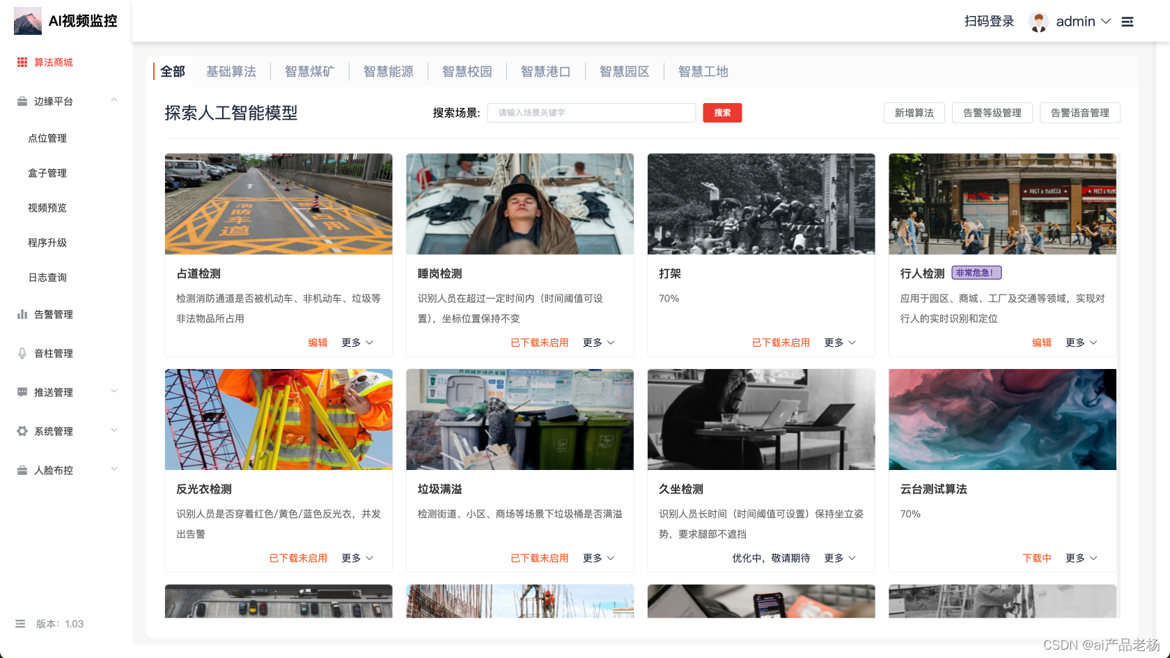
自动学习和优化过程,实现更加精准的预测和决策的智慧交通开源了
智慧交通视觉监控平台是一款功能强大且简单易用的实时算法视频监控系统。它的愿景是最底层打通各大芯片厂商相互间的壁垒,省去繁琐重复的适配流程,实现芯片、算法、应用的全流程组合,从而大大减少企业级应用约95%的开发成本。通过高效的实时视…

DeepSeek R1 本地部署指南 (3) - 更换本地部署模型 Windows/macOS 通用
0.准备 完成 Windows 或 macOS 安装: DeepSeek R1 本地部署指南 (1) - Windows 本地部署-CSDN博客 DeepSeek R1 本地部署指南 (2) - macOS 本地部署-CSDN博客 以下内容 Windows 和 macOS 命令执行相同: Windows 管理员启动:命令提示符 CMD ma…
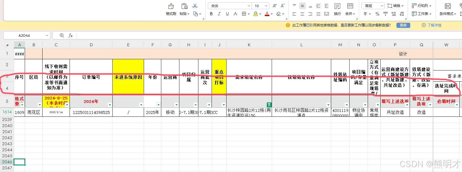
使用 Node.js 读取 Excel 文件并处理合并单元格
使用 Node.js 读取 Excel 文件并处理合并单元格
在现代的数据处理任务中,Excel 文件是一种非常常见的数据存储格式。无论是数据分析、报表生成,还是数据迁移,Excel 文件都扮演着重要的角色。然而,处理 Excel 文件时,尤…

汇川EASY系列之以太网通讯(MODBUS_TCP做从站)
汇川easy系列PLC做MODBUS_TCP从站,不需要任何操作,但是有一些需要知道的东西。具体如下:
1、汇川easy系列PLC做MODBUS_TCP从站,,ModbusTCP服务器默认开启,无需设置通信协议(即不需要配置),端口号为“502”。ModbusTCP从站最多支持31个ModbusTCP客户端(ModbusTCP主站…

1996-2023年各省公路里程数据(无缺失)
1996-2023年各省公路里程数据(无缺失)
1、时间:1996-2023年
2、来源:国家统计局、统计年鉴
3、指标:公路里程(万公里)
4、范围:31省
5、指标解释:公路里程指报告期末…


从“不敢买大”到“按墙选屏”,海信电视如何凭百吋重构客厅?
电视买小了,成为茜茜新房入住后最大的遗憾。
新房装修的时候,茜茜担心电视买大了眼睛看着累,因此把尺寸选在了65吋。结果入住后,孩子看动画片嚷着“画面太小”,老公看球赛吐槽“看不清球员号码”,全家追剧…

Swift 经典链表面试题:如何在不访问头节点的情况下删除指定节点?
摘要
在日常开发中,链表虽然不像数组、字典那么常用,但在某些场景下还是挺重要的。尤其是面试的时候,链表题目可是经典考点之一。今天我们要聊的就是一个看似简单,但很多人第一次做都会卡住的问题——删除单链表中的指定节点。
…

楼宇自控系统的结构密码:总线与分布式结构方式的差异与应用
在现代建筑中,为了实现高效、智能的管理,楼宇自控系统变得越来越重要。它就像建筑的 智能管家,可自动控制照明、空调、通风等各种机电设备,让建筑运行更顺畅,还能节省能源成本。而在楼宇自控系统里,有两种关…
![git | 回退版本 并保存当前修改到stash,在进行整合。[git checkout | git stash 等方法 ]](https://i-blog.csdnimg.cn/direct/ee00457b8a034146abd41f436cffe983.png)
git | 回退版本 并保存当前修改到stash,在进行整合。[git checkout | git stash 等方法 ]
目录
一些常见命令:
git 回退版本
一、临时回退(不会修改历史,可随时回到当前版本)
方法1:git checkout HEAD~1
问题:处于 detached HEAD 状态下提交的,无法直接 git push
✅ 选项 1&…

Linux系统之美:环境变量的概念以及基本操作
本节重点 理解环境变量的基本概念学会在指令和代码操作上查询更改环境变量环境变量表的基本概念父子进程间环境变量的继承与隔离 一、引入
1.1 自定义命令(我们的exe) 我们以往的Linux编程经验告诉我们,我们在对一段代码编译形成可执行文件后…
推荐文章
- mysql下载与安装、关系数据库和表的创建
- 抖音生活服务加强探店内容治理,2024年达人违规率下降30%
- (十 一)趣学设计模式 之 组合模式!
- (一)Axure制作移动端登录页面
- (一)相机标定——四大坐标系的介绍、对应转换、畸变原理以及OpenCV完整代码实战(C++版)
- [AI]从零开始的llama.cpp部署与DeepSeek格式转换、量化、运行教程
- “harmony”整合不同平台的单细胞数据之旅
- 《A++ 敏捷开发》- 18 软件需求
- 《南京日报》专题报道 | 耘瞳科技“工业之眼”加码“中国智造”
- 「vue3-element-admin」告别 vite-plugin-svg-icons!用 @unocss/preset-icons 加载本地 SVG 图标
- 【10】单片机编程核心技巧:指令周期与晶振频率
- 【AI News | 20250316】每日AI进展