Stacked Regressions : Top 4% on LeaderBoard

• Pedro Marcelino用Python进行全面的数据探索：伟大的、非常有动机的数据分析 Julien Cohen
• Solal在Ames数据集回归研究中的应用：深入研究线性回归分析的彻底特征，但对初学者来说非常容易理解。
• Alexandru Papiu的正则化线性模型：建模和交叉验证的最佳初始内核

选用堆叠模型，构建了两个堆栈类（最简单的方法和不太简单的方法）。
特征工程优点：

• 通过按顺序处理数据来估算缺失值
• 转换一些看起来很明确的数值变量
• 编码某些类别变量的标签，这些变量的排序集中可能包含信息
• 倾斜特征的Box-Cox转换（而不是log转换）：在排行榜和交叉验证上结果较好
• 获取分类特征的虚拟变量。

选择多个基本模型（主要是基于sklearn的模型以及sklearn API的DMLC的XGBoost和微软的LightGBM），先交叉验证，然后叠加/集成。关键是使（线性）模型对异常值具有鲁棒性。这改善了LB和交叉验证的结果。

1. 数据读取

#import some necessary librairiesimport numpy as np # linear algebra
import pandas as pd # data processing, CSV file I/O (e.g. pd.read_csv)
%matplotlib inline
import matplotlib.pyplot as plt  # Matlab-style plotting
import seaborn as sns
color = sns.color_palette()
sns.set_style('darkgrid')
import warnings
def ignore_warn(*args, **kwargs):passwarnings.warn = ignore_warn #ignore annoying warning (from sklearn and seaborn)from scipy import stats
from scipy.stats import norm, skew #for some statisticspd.set_option('display.float_format', lambda x: '{:.3f}'.format(x)) #Limiting floats output to 3 decimal pointsfrom subprocess import check_output
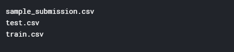
print(check_output(["ls", "../input"]).decode("utf8")) #check the files available in the directory

读取数据

#读取数据
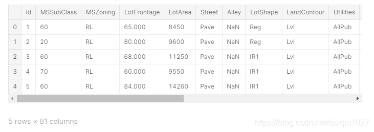
train = pd.read_csv('../input/train.csv')
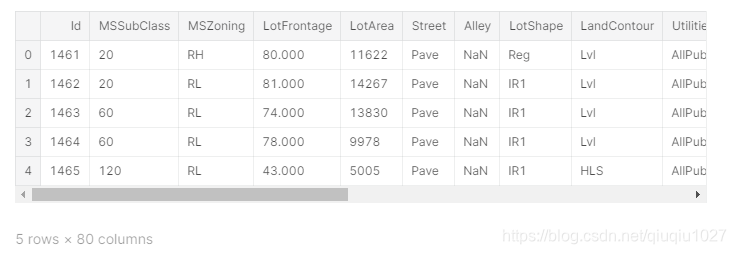
test = pd.read_csv('../input/test.csv')

查看前5行

train.head(5)

test.head(5)

检查样本和特征的数量

#check the numbers of samples and features
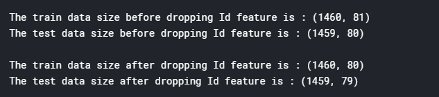
print("The train data size before dropping Id feature is : {} ".format(train.shape))
print("The test data size before dropping Id feature is : {} ".format(test.shape))#Save the 'Id' column
train_ID = train['Id']
test_ID = test['Id']#Now drop the  'Id' colum since it's unnecessary for  the prediction process.
train.drop("Id", axis = 1, inplace = True)
test.drop("Id", axis = 1, inplace = True)#check again the data size after dropping the 'Id' variable
print("\nThe train data size after dropping Id feature is : {} ".format(train.shape)) 
print("The test data size after dropping Id feature is : {} ".format(test.shape))

2. 数据处理

异常值

fig, ax = plt.subplots()
ax.scatter(x = train['GrLivArea'], y = train['SalePrice'])
plt.ylabel('SalePrice', fontsize=13)
plt.xlabel('GrLivArea', fontsize=13)
plt.show()

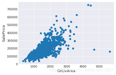
右下角看到两个巨大的grlivrea，价格很低。

#Deleting outliers
train = train.drop(train[(train['GrLivArea']>4000) & (train['SalePrice']<300000)].index)#Check the graphic again
fig, ax = plt.subplots()
ax.scatter(train['GrLivArea'], train['SalePrice'])
plt.ylabel('SalePrice', fontsize=13)
plt.xlabel('GrLivArea', fontsize=13)
plt.show()

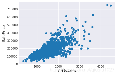
注：

异常值的移除是安全的。我们决定删除这两个，因为它们是非常巨大和非常糟糕的（非常大的面积，非常低的价格）。
训练数据中可能还有其他异常值。但是，如果测试数据中也存在异常值，那么删除所有这些异常值可能会严重影响我们的模型。这就是为什么，我们不把它们全部删除，而只是设法使我们的一些模型在它们上更加健壮。可以参考模型部分。

目标变量
需要预测SalePrice，所以先分析它

sns.distplot(train['SalePrice'] , fit=norm);# Get the fitted parameters used by the function
(mu, sigma) = norm.fit(train['SalePrice'])
print( '\n mu = {:.2f} and sigma = {:.2f}\n'.format(mu, sigma))#Now plot the distribution
plt.legend(['Normal dist. ($\mu=$ {:.2f} and $\sigma=$ {:.2f} )'.format(mu, sigma)],loc='best')
plt.ylabel('Frequency')
plt.title('SalePrice distribution')#Get also the QQ-plot
fig = plt.figure()
res = stats.probplot(train['SalePrice'], plot=plt)
plt.show()

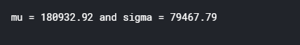
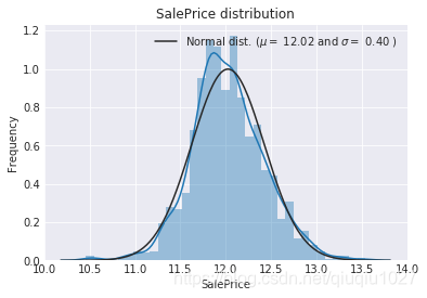
目标变量向右倾斜。由于（线性）模型喜欢正态分布的数据，我们需要转换这个变量，使其更为正态分布。

目标变量的对数变换

#We use the numpy fuction log1p which  applies log(1+x) to all elements of the column
train["SalePrice"] = np.log1p(train["SalePrice"])#Check the new distribution 
sns.distplot(train['SalePrice'] , fit=norm);# Get the fitted parameters used by the function
(mu, sigma) = norm.fit(train['SalePrice'])
print( '\n mu = {:.2f} and sigma = {:.2f}\n'.format(mu, sigma))#Now plot the distribution
plt.legend(['Normal dist. ($\mu=$ {:.2f} and $\sigma=$ {:.2f} )'.format(mu, sigma)],loc='best')
plt.ylabel('Frequency')
plt.title('SalePrice distribution')#Get also the QQ-plot
fig = plt.figure()
res = stats.probplot(train['SalePrice'], plot=plt)
plt.show()

特征工程

连接训练集和测试集

ntrain = train.shape[0]
ntest = test.shape[0]
y_train = train.SalePrice.values
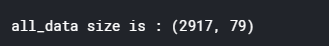
all_data = pd.concat((train, test)).reset_index(drop=True)
all_data.drop(['SalePrice'], axis=1, inplace=True)
print("all_data size is : {}".format(all_data.shape))

缺失值

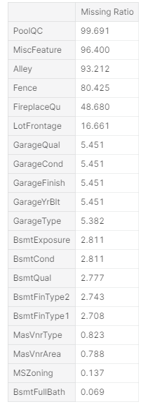
all_data_na = (all_data.isnull().sum() / len(all_data)) * 100
all_data_na = all_data_na.drop(all_data_na[all_data_na == 0].index).sort_values(ascending=False)[:30]
missing_data = pd.DataFrame({'Missing Ratio' :all_data_na})
missing_data.head(20)

f, ax = plt.subplots(figsize=(15, 12))
plt.xticks(rotation='90')
sns.barplot(x=all_data_na.index, y=all_data_na)
plt.xlabel('Features', fontsize=15)
plt.ylabel('Percent of missing values', fontsize=15)
plt.title('Percent missing data by feature', fontsize=15)

相关性

#Correlation map to see how features are correlated with SalePrice
corrmat = train.corr()
plt.subplots(figsize=(12,9))
sns.heatmap(corrmat, vmax=0.9, square=True)

估算缺失值
我们通过依次处理缺失值的特征来估算它们

• PoolQC：NA表示“没有泳池”。这是有道理的，因为丢失价值的比例很高（+99%），而且大多数房子根本没有游泳池

all_data["PoolQC"] = all_data["PoolQC"].fillna("None")

• MiscFeature : NA 表示“没有混合特性”

all_data["MiscFeature"] = all_data["MiscFeature"].fillna("None")

• Alley : NA 表示“没有巷子通道”

all_data["Alley"] = all_data["Alley"].fillna("None")

• Fence : NA 表示“没有围栏”

all_data["Fence"] = all_data["Fence"].fillna("None")

• FireplaceQu : NA 表示“没有壁炉”

all_data["FireplaceQu"] = all_data["FireplaceQu"].fillna("None")

• LotFrontage : 由于与房产相连的每条街道的面积很可能与其附近的其他房屋面积相似，因此我们可以通过该街区的中间地块面积来填充缺失值。

#Group by neighborhood and fill in missing value by the median LotFrontage of all the neighborhood
all_data["LotFrontage"] = all_data.groupby("Neighborhood")["LotFrontage"].transform(lambda x: x.fillna(x.median()))

• GarageType, GarageFinish, GarageQual and GarageCond : 用“None”代替缺失值

for col in ('GarageType', 'GarageFinish', 'GarageQual', 'GarageCond'):all_data[col] = all_data[col].fillna('None')

• GarageYrBlt, GarageArea and GarageCars :将缺失数据替换为0（因为没有车库=此类车库中没有汽车。）

for col in ('GarageYrBlt', 'GarageArea', 'GarageCars'):all_data[col] = all_data[col].fillna(0)

• BsmtFinSF1, BsmtFinSF2, BsmtUnfSF, TotalBsmtSF, BsmtFullBath and BsmtHalfBath : 由于没有地下室，缺失值值可能为零

for col in ('BsmtFinSF1', 'BsmtFinSF2', 'BsmtUnfSF','TotalBsmtSF', 'BsmtFullBath', 'BsmtHalfBath'):all_data[col] = all_data[col].fillna(0)

• BsmtQual, BsmtCond, BsmtExposure, BsmtFinType1 and BsmtFinType2 :对于所有这些与地下室相关的分类特征，NaN意味着没有地下室。

for col in ('BsmtQual', 'BsmtCond', 'BsmtExposure', 'BsmtFinType1', 'BsmtFinType2'):all_data[col] = all_data[col].fillna('None')

• MasVnrArea and MasVnrType : NA 很可能意味着这些房子没有砖石饰面。我们可以为区域填充0，为类型填充None

all_data["MasVnrType"] = all_data["MasVnrType"].fillna("None")
all_data["MasVnrArea"] = all_data["MasVnrArea"].fillna(0)

• MSZoning （一般分区分类）：“RL”是最常见的值。所以我们可以用“RL”填充缺失的值

all_data['MSZoning'] = all_data['MSZoning'].fillna(all_data['MSZoning'].mode()[0])

• Utilities : 对于这个分类特征，所有记录都是“AllPub”，除了一个“NoSeWa”和两个NA。因为有“NoSewa”的房子在训练集中，这个特性对预测建模没有帮助。然后我们可以安全地移除它。

all_data = all_data.drop(['Utilities'], axis=1)

• Functional : NA 意味着典型

all_data["Functional"] = all_data["Functional"].fillna("Typ")

• Electrical : 它有一个NA值。由于这个特性主要是’SBrkr’，可以将缺失值设置为此。

all_data['Electrical'] = all_data['Electrical'].fillna(all_data['Electrical'].mode()[0])

• KitchenQual: 只有一个NA值，和Electrical一样，我们为KitchenQual中丢失的值设置“TA”（最常见）。

all_data['KitchenQual'] = all_data['KitchenQual'].fillna(all_data['KitchenQual'].mode()[0])

• Exterior1st and Exterior2nd : 同样，外部1和2只有一个缺失值。我们将用最常用的字符串替换

all_data['Exterior1st'] = all_data['Exterior1st'].fillna(all_data['Exterior1st'].mode()[0])
all_data['Exterior2nd'] = all_data['Exterior2nd'].fillna(all_data['Exterior2nd'].mode()[0])

• SaleType :用最频繁的 "WD"填充

all_data['SaleType'] = all_data['SaleType'].fillna(all_data['SaleType'].mode()[0])

• MSSubClass : Na 很可能意味着没有建筑类。我们可以用None替换缺失值

all_data['MSSubClass'] = all_data['MSSubClass'].fillna("None")

检查还有没有缺失值

#Check remaining missing values if any 
all_data_na = (all_data.isnull().sum() / len(all_data)) * 100
all_data_na = all_data_na.drop(all_data_na[all_data_na == 0].index).sort_values(ascending=False)
missing_data = pd.DataFrame({'Missing Ratio' :all_data_na})
missing_data.head()

更多特征工程

转换一些真正分类的数值变量

#MSSubClass=The building class
all_data['MSSubClass'] = all_data['MSSubClass'].apply(str)#Changing OverallCond into a categorical variable
all_data['OverallCond'] = all_data['OverallCond'].astype(str)#Year and month sold are transformed into categorical features.
all_data['YrSold'] = all_data['YrSold'].astype(str)
all_data['MoSold'] = all_data['MoSold'].astype(str)

编码某些类别变量的标签，这些变量的排序集中可能包含信息

from sklearn.preprocessing import LabelEncoder
cols = ('FireplaceQu', 'BsmtQual', 'BsmtCond', 'GarageQual', 'GarageCond', 'ExterQual', 'ExterCond','HeatingQC', 'PoolQC', 'KitchenQual', 'BsmtFinType1', 'BsmtFinType2', 'Functional', 'Fence', 'BsmtExposure', 'GarageFinish', 'LandSlope','LotShape', 'PavedDrive', 'Street', 'Alley', 'CentralAir', 'MSSubClass', 'OverallCond', 'YrSold', 'MoSold')
# process columns, apply LabelEncoder to categorical features
for c in cols:lbl = LabelEncoder() lbl.fit(list(all_data[c].values)) all_data[c] = lbl.transform(list(all_data[c].values))# shape        
print('Shape all_data: {}'.format(all_data.shape))

添加一个更重要的特征

由于区域相关特征对房价的决定非常重要，我们又增加了一个特征，即每套房子的地下室、一楼和二楼的总面积

# Adding total sqfootage feature 
all_data['TotalSF'] = all_data['TotalBsmtSF'] + all_data['1stFlrSF'] + all_data['2ndFlrSF']

倾斜特征

numeric_feats = all_data.dtypes[all_data.dtypes != "object"].index# Check the skew of all numerical features
skewed_feats = all_data[numeric_feats].apply(lambda x: skew(x.dropna())).sort_values(ascending=False)
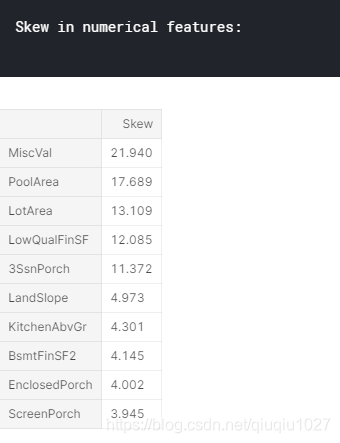
print("\nSkew in numerical features: \n")
skewness = pd.DataFrame({'Skew' :skewed_feats})
skewness.head(10)

（高度）倾斜特征的Box-Cox变换
使用scipy函数boxcox1p计算1+x的Box-Cox变换。
请注意，设置λ=0相当于上述用于目标变量的log1p。
有关Box-Cox转换和scipy函数页的详细信息，请参见本页

skewness = skewness[abs(skewness) > 0.75]
print("There are {} skewed numerical features to Box Cox transform".format(skewness.shape[0]))from scipy.special import boxcox1p
skewed_features = skewness.index
lam = 0.15
for feat in skewed_features:#all_data[feat] += 1all_data[feat] = boxcox1p(all_data[feat], lam)#all_data[skewed_features] = np.log1p(all_data[skewed_features])

获取虚拟分类特征

all_data = pd.get_dummies(all_data)
print(all_data.shape)

新的训练集与测试集

train = all_data[:ntrain]
test = all_data[ntrain:]

3. 建模

导入库

from sklearn.linear_model import ElasticNet, Lasso,  BayesianRidge, LassoLarsIC
from sklearn.ensemble import RandomForestRegressor,  GradientBoostingRegressor
from sklearn.kernel_ridge import KernelRidge
from sklearn.pipeline import make_pipeline
from sklearn.preprocessing import RobustScaler
from sklearn.base import BaseEstimator, TransformerMixin, RegressorMixin, clone
from sklearn.model_selection import KFold, cross_val_score, train_test_split
from sklearn.metrics import mean_squared_error
import xgboost as xgb
import lightgbm as lgb

定义交叉验证策略

使用Sklearn的cross-valu-score函数。但是这个函数没有shuffle属性，我们添加一行代码，以便在交叉验证之前对数据集进行shuffle

#Validation function
n_folds = 5def rmsle_cv(model):kf = KFold(n_folds, shuffle=True, random_state=42).get_n_splits(train.values)rmse= np.sqrt(-cross_val_score(model, train.values, y_train, scoring="neg_mean_squared_error", cv = kf))return(rmse)

基本模型

1）LASSO回归：

这个模型可能对异常值非常敏感。所以我们需要让它对他们更加有力。为此，使用sklearn的Robustscaler（）方法

lasso = make_pipeline(RobustScaler(), Lasso(alpha =0.0005, random_state=1))

2）Elastic Net Regression（弹性网回归）：

再次对异常值保持稳健

ENet = make_pipeline(RobustScaler(), ElasticNet(alpha=0.0005, l1_ratio=.9, random_state=3))

3）Kernel Ridge Regression（核岭回归） :

KRR = KernelRidge(alpha=0.6, kernel='polynomial', degree=2, coef0=2.5)

4）Gradient Boosting Regression （梯度增强回归）：

由于huber损失使得它对异常值很稳健:

GBoost = GradientBoostingRegressor(n_estimators=3000, learning_rate=0.05,max_depth=4, max_features='sqrt',min_samples_leaf=15, min_samples_split=10, loss='huber', random_state =5)

5）XGBoost :

model_xgb = xgb.XGBRegressor(colsample_bytree=0.4603, gamma=0.0468, learning_rate=0.05, max_depth=3, min_child_weight=1.7817, n_estimators=2200,reg_alpha=0.4640, reg_lambda=0.8571,subsample=0.5213, silent=1,random_state =7, nthread = -1)

6）LightGBM :

model_lgb = lgb.LGBMRegressor(objective='regression',num_leaves=5,learning_rate=0.05, n_estimators=720,max_bin = 55, bagging_fraction = 0.8,bagging_freq = 5, feature_fraction = 0.2319,feature_fraction_seed=9, bagging_seed=9,min_data_in_leaf =6, min_sum_hessian_in_leaf = 11)

基本模型得分

通过评估交叉验证rmsle错误来了解这些基本模型是如何对执行数据

score = rmsle_cv(lasso)
print("\nLasso score: {:.4f} ({:.4f})\n".format(score.mean(), score.std()))

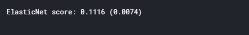
score = rmsle_cv(ENet)
print("ElasticNet score: {:.4f} ({:.4f})\n".format(score.mean(), score.std()))

score = rmsle_cv(KRR)
print("Kernel Ridge score: {:.4f} ({:.4f})\n".format(score.mean(), score.std()))

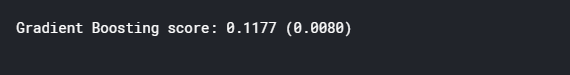
score = rmsle_cv(GBoost)
print("Gradient Boosting score: {:.4f} ({:.4f})\n".format(score.mean(), score.std()))

score = rmsle_cv(model_xgb)
print("Xgboost score: {:.4f} ({:.4f})\n".format(score.mean(), score.std()))

score = rmsle_cv(model_lgb)
print("LGBM score: {:.4f} ({:.4f})\n" .format(score.mean(), score.std()))

叠加模型

最简单的叠加方法：平均基本模型

从平均基本模型的简单方法开始。构建了一个新的类，用我们的模型扩展scikit-learn，还扩展了laverage封装和代码重用（继承）

平均基本模型类

class AveragingModels(BaseEstimator, RegressorMixin, TransformerMixin):def __init__(self, models):self.models = models# we define clones of the original models to fit the data indef fit(self, X, y):self.models_ = [clone(x) for x in self.models]# Train cloned base modelsfor model in self.models_:model.fit(X, y)return self#Now we do the predictions for cloned models and average themdef predict(self, X):predictions = np.column_stack([model.predict(X) for model in self.models_])return np.mean(predictions, axis=1)   

平均基本模型得分

在这平均了四个模型，ENet, GBoost, KRR 和lasso。当然，也可以添加更多的模型。

averaged_models = AveragingModels(models = (ENet, GBoost, KRR, lasso))score = rmsle_cv(averaged_models)
print(" Averaged base models score: {:.4f} ({:.4f})\n".format(score.mean(), score.std()))

即使是最简单的叠加方法也能真正提高分数。这鼓励我们进一步探索一种不那么简单的堆叠方法。

不那么简单的叠加：添加元模型

在这种方法中，我们在平均基本模型上添加一个元模型，并使用这些基本模型的折叠预测来训练我们的元模型。

训练部分的程序可描述如下：

1. 将整个训练集分成两个不相交的集（这里是train和holdout）
2. 在第一部分（train）上训练几个基本模型
3. 在第二部分测试这些基本模型（holdout）
4. 使用来自第三步的预测（称为折叠预测）作为输入，并使用正确的响应（目标变量）作为输出，以训练称为元模型的高级学习者。

前三步是迭代完成的。以5倍叠加为例，首先将训练数据分成5倍。然后进行5次迭代。在每次迭代中，将每个基本模型训练为4个折叠，并预测剩余折叠（保持折叠）。

因此，在5次迭代之后，整个数据将被用于获得折叠预测，然后将在步骤4中使用这些预测作为新特性来训练元模型。

在预测部分，根据测试数据对所有基本模型的预测进行平均，并将其作为元特征，在此基础上利用元模型进行最终预测。

叠加平均模型类

class StackingAveragedModels(BaseEstimator, RegressorMixin, TransformerMixin):def __init__(self, base_models, meta_model, n_folds=5):self.base_models = base_modelsself.meta_model = meta_modelself.n_folds = n_folds# We again fit the data on clones of the original modelsdef fit(self, X, y):self.base_models_ = [list() for x in self.base_models]self.meta_model_ = clone(self.meta_model)kfold = KFold(n_splits=self.n_folds, shuffle=True, random_state=156)# Train cloned base models then create out-of-fold predictions# that are needed to train the cloned meta-modelout_of_fold_predictions = np.zeros((X.shape[0], len(self.base_models)))for i, model in enumerate(self.base_models):for train_index, holdout_index in kfold.split(X, y):instance = clone(model)self.base_models_[i].append(instance)instance.fit(X[train_index], y[train_index])y_pred = instance.predict(X[holdout_index])out_of_fold_predictions[holdout_index, i] = y_pred# Now train the cloned  meta-model using the out-of-fold predictions as new featureself.meta_model_.fit(out_of_fold_predictions, y)return self#Do the predictions of all base models on the test data and use the averaged predictions as #meta-features for the final prediction which is done by the meta-modeldef predict(self, X):meta_features = np.column_stack([np.column_stack([model.predict(X) for model in base_models]).mean(axis=1)for base_models in self.base_models_ ])return self.meta_model_.predict(meta_features)

叠加平均模型得分

为了使这两种方法具有可比性（通过使用相同数量的模型），只需平均Enet KRR和Gboost，然后添加lasso作为元模型。

stacked_averaged_models = StackingAveragedModels(base_models = (ENet, GBoost, KRR),meta_model = lasso)score = rmsle_cv(stacked_averaged_models)
print("Stacking Averaged models score: {:.4f} ({:.4f})".format(score.mean(), score.std()))

通过增加元学习者，又得到了更好的分数

StackedRegressor、XGBoost和LightGBM，将XGBoost和LightGBM添加到前面定义的StackedRegressor中。

首先定义一个rmsle评估函数

def rmsle(y, y_pred):return np.sqrt(mean_squared_error(y, y_pred))

最后训练和预测

• StackedRegressor

stacked_averaged_models.fit(train.values, y_train)
stacked_train_pred = stacked_averaged_models.predict(train.values)
stacked_pred = np.expm1(stacked_averaged_models.predict(test.values))
print(rmsle(y_train, stacked_train_pred))

• XGBoost:

model_xgb.fit(train, y_train)
xgb_train_pred = model_xgb.predict(train)
xgb_pred = np.expm1(model_xgb.predict(test))
print(rmsle(y_train, xgb_train_pred))

• LightGBM:

model_lgb.fit(train, y_train)
lgb_train_pred = model_lgb.predict(train)
lgb_pred = np.expm1(model_lgb.predict(test.values))
print(rmsle(y_train, lgb_train_pred))

'''RMSE on the entire Train data when averaging'''print('RMSLE score on train data:')
print(rmsle(y_train,stacked_train_pred*0.70 +xgb_train_pred*0.15 + lgb_train_pred*0.15 ))

集合预测:

ensemble = stacked_pred*0.70 + xgb_pred*0.15 + lgb_pred*0.15

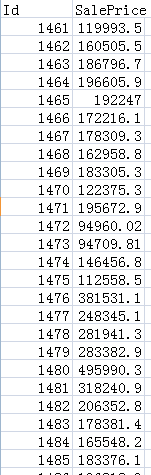
输出

sub = pd.DataFrame()
sub['Id'] = test_ID
sub['SalePrice'] = ensemble
sub.to_csv('submission.csv',index=False)