作业二

文章目录（嫌墨迹可以直接点击目录跳转到源代码查看）

文章目录

作业二
第一题
- 1.1 数据可视化
- - 代码
  - 讲解
  - 结果
- 1.2 实现
- - 1.2.1 热身运动 sigmoid 函数
  - - 代码
  - 1.2.2 损失函数和梯度
  - - 代码
    - 结果
    - 思路
  - 1.2.3 手动梯度下降尝试学习参数
  - - 代码
    - 结果
    - 总结
  - 1.2.3 使用fminunc函数来进行参数的学习
  - - 代码
    - 结果
    - 思路
  - 1.2.4
  - - 代码
    - 结果
    - 思路
- 源代码
第二题
- 2.1 数据可视化
- - 代码
  - 结果
  - 讲解
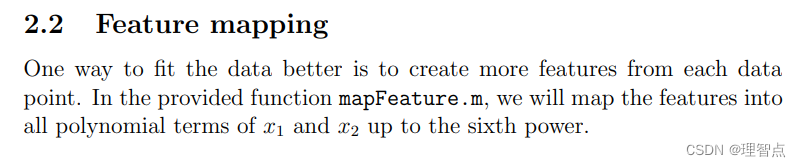
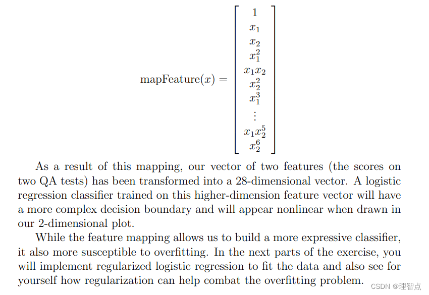
- 2.2 特征值映射
- - 代码
  - 讲解
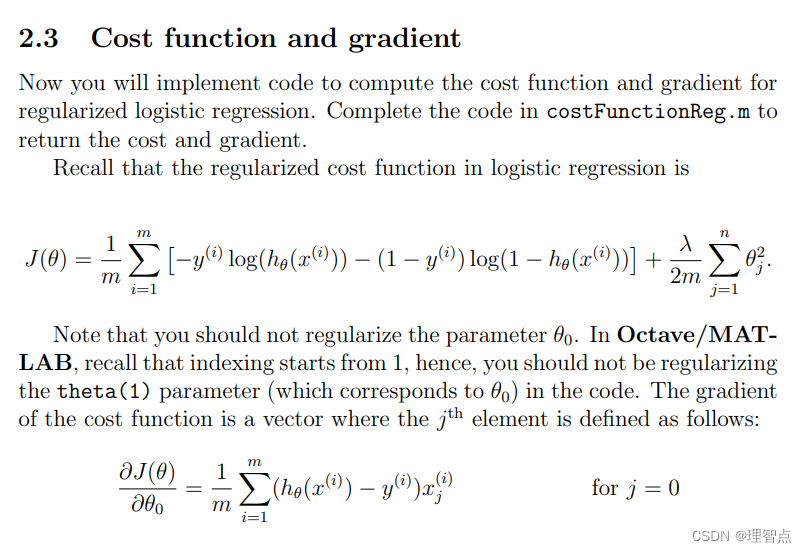
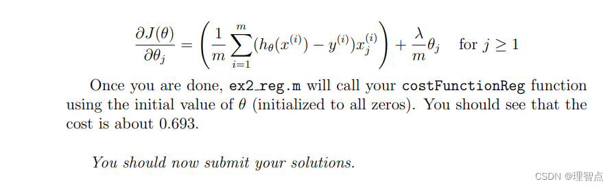
- 2.3 损失函数及其梯度
- - 代码
  - 讲解
- 2.3.1 使用fuminc进行参数拟合
- - 代码
  - 讲解
- 2.4 绘制决策边界
- - 代码
  - 结果
  - 讲解
- 2.5 可选练习（尝试不同的Lambda值）
- - 讲解
- 源代码

第一题

1.1 数据可视化

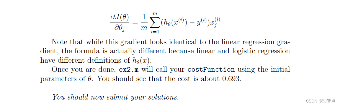
英文题面
在这里插入图片描述
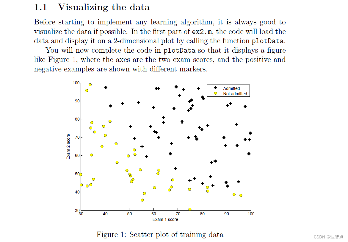
大致翻译：
在开始实施任何学习算法之前，最好如果可能的话，将数据可视化。在ex2.m的第一部分中，代码将加载数据，并通过调用函数plotData将其显示在二维绘图上。现在，您将完成plotData中的代码，以便它显示一个图形如图1所示，轴是两个考试分数，通过和不通过的例子显示了不同的标记。

代码

import numpy as np
import matplotlib.pyplot as plt
import pandas as pdexam1_score_label = 'Exam1 Score'
exam2_score_label = 'Exam2 Score'
admitted_label = 'Admitted'
# 读取数据
datas = pd.read_csv("./ex2data1.txt", header=None, names=[exam1_score_label, exam2_score_label, admitted_label])
# 获取数据个数
m = len(datas)
#将数据分类用于绘图
positive = datas[datas[admitted_label].isin([1])]
negative = datas[datas[admitted_label].isin([0])]
# 绘图
plt.scatter(x=positive[exam1_score_label], y=positive[exam2_score_label], marker='o', label='Admitted', color='g')
plt.scatter(x=negative[exam1_score_label], y=negative[exam2_score_label], marker='x', label="Not Admitted", color='r')plt.legend()
plt.xlabel(exam1_score_label)
plt.ylabel(exam2_score_label)
plt.show()

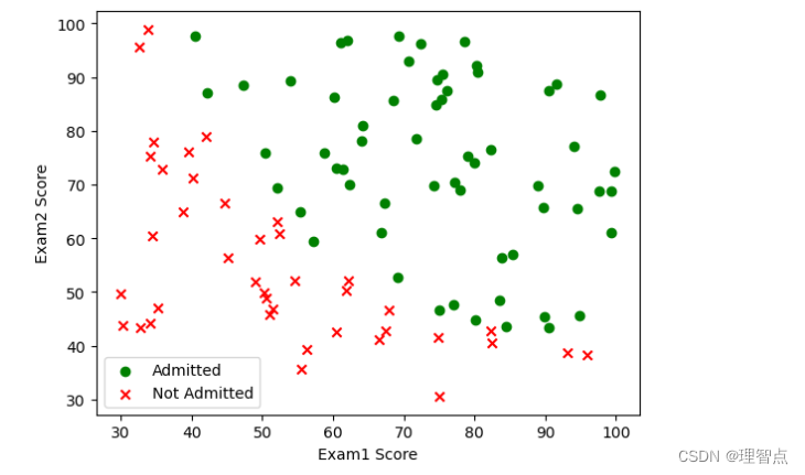
讲解

使用pandas读取数据，并对数据进行分类，然后进行画图，要画出不同的标记点的图
重要的是plt.scatter()函数中传递的参数marker,具体的参数表可以看这篇文章

这里有一点需要注意，妈的这个marker传递不了数组，所以在我的代码之中我用了两次plt.scatter来绘制两种图形，我一开始想的是将marker传递一个数组
如 marker = [‘o’ if item == 1else ‘x’ for item in datas[admitted_label] ]，
然后绘制出对应的图形，节省点代码量，但是不行。我花了好久才确定这件事是不可行的，为什么会花了好长时间确定呢，因为chatGpt跟我说可以，但是我实际测试不行，最后迫不得已用了两次scatter

结果

在这里插入图片描述

1.2 实现

1.2.1 热身运动 sigmoid 函数

题面
在这里插入图片描述
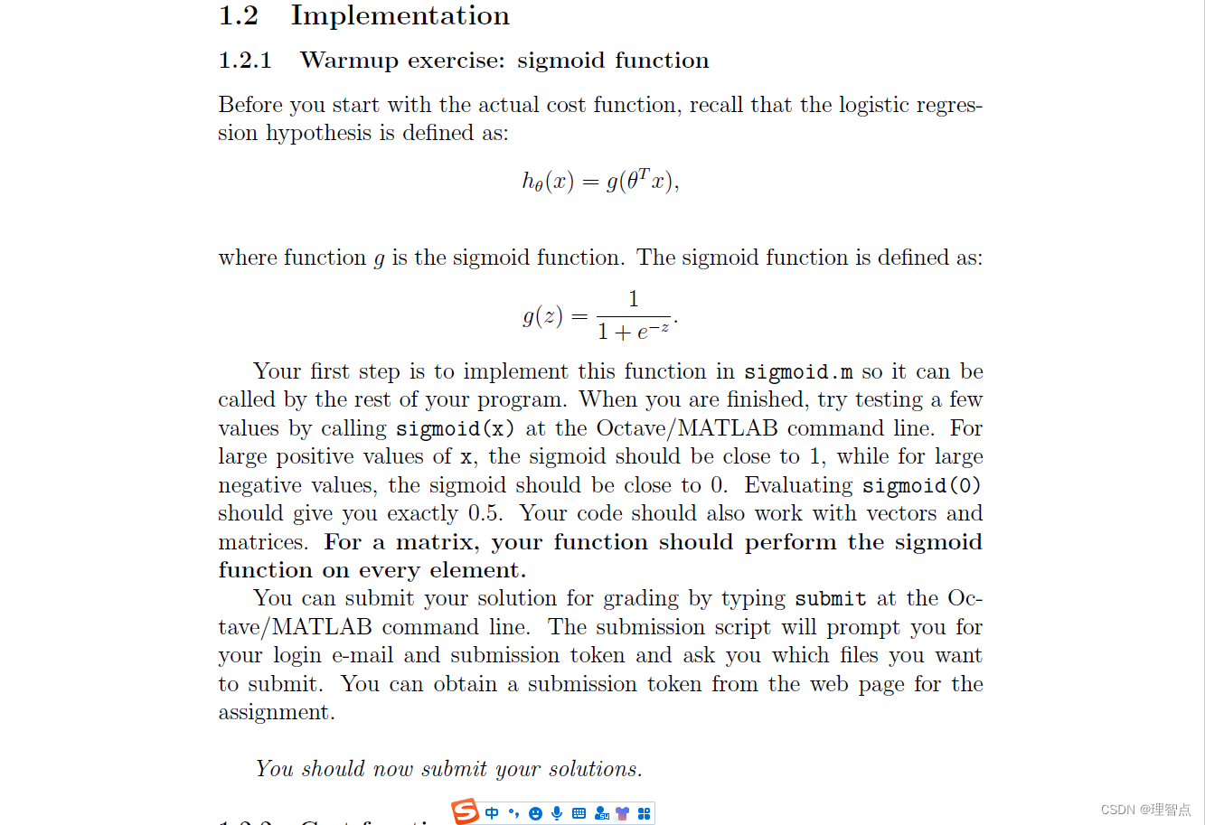
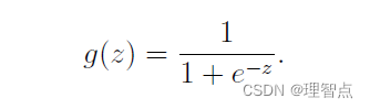
这里就是让我们实现sigmoid函数

代码

先处理一下数据

# 处理数据# 这个判断防止调试脚本的时候多次插入bias行
if 'bias' not in datas.columns:datas.insert(0, 'bias', 1)
datas.head()
x = np.matrix(datas.iloc[:, 0:3])
y = np.matrix(datas.iloc[:, 3:4])
# theta = np.matrix(np.zeros(x.shape[1]))
theta = np.zeros((x.shape[1], 1))

定义预测函数和sigmoid函数

# 定义预测函数
def h_fun(x_param, theta_param):return sigmoid(x_param @ theta_param)# 定义sigmoid函数
def sigmoid(z_param):return 1 / (1 + np.exp(-z_param))

1.2.2 损失函数和梯度

在这里插入图片描述

代码

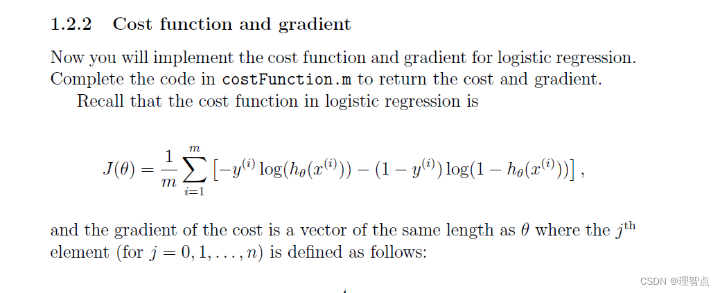
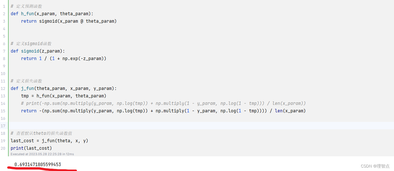
这里让我们进行一次损失函数的计算

# 定义损失函数
def j_fun(theta_param, x_param, y_param):tmp = h_fun(x_param, theta_param)# print(-np.sum(np.multiply(y_param, np.log(tmp)) + np.multiply(1 - y_param, np.log(1 - tmp))) / len(x_param))return -(np.sum(np.multiply(y_param, np.log(tmp)) + np.multiply(1 - y_param, np.log(1 - tmp)))) / len(x_param)# 查看默认theta的损失函数值
last_cost = j_fun(theta, x, y)
print(last_cost)

结果

在这里插入图片描述

思路

这个没啥好说的，都是按部就班的跟着作业要求来

1.2.3 手动梯度下降尝试学习参数

在按照题目要求使用fminunc进行参数的学习之前，我们先手动进行下之前学会的梯度下降来进行参数的学习（为什么这么做呢，就是为了体验，闲的，如果你不想尝试，可以直接略过）

先自己写一个梯度下降函数

代码

# 自己写梯度下降
def gradient_descent(alpha, iteration, train_x, train_y, train_theta):for i in range(iteration):tmp = h_fun(train_x, train_theta)train_theta = train_theta - (alpha / m) * (train_x.T @ (tmp - train_y))return train_theta

gradient_descent函数的几个参数含义我放在下面了

参数	释义
alpha	学习速度
iteration	学习次数
train_x	x
train_y	y
train_theta	需训练参数

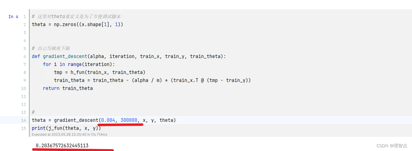
完整代码如下,我先对学习速度和学习次数进行模糊了，你先自己手动尝试梯度下降的调参，我提前告诉你最后学习出来的参数的损失函数值是 0.203*******，最后我挑出来的参数会放在结果中

# 这里对theta重定义是为了方便调试脚本
theta = np.zeros((x.shape[1], 1))# 自己写梯度下降
def gradient_descent(alpha, iteration, train_x, train_y, train_theta):for i in range(iteration):tmp = h_fun(train_x, train_theta)train_theta = train_theta - (alpha / m) * (train_x.T @ (tmp - train_y))return train_theta#请在****处补充你的学习速度和学习次数
theta = gradient_descent(****, ******, x, y, theta)
print(j_fun(theta, x, y))

结果

在这里插入图片描述

总结

如果你自己尝试了手动进行梯度下降，你就会知道这个调参的过程很烦，当然，你可以把梯度下降写的更好一点，比如说对学习速度alpha 进行动态变更等等操作，但是，总的来说都是比较麻烦的一个过程。因此我们要借鉴前人的智慧，调包！

1.2.3 使用fminunc函数来进行参数的学习

因为我们使用的是Python环境，所以我们使用scipy.optimize包中的fmin_tnc函数来实现

代码

# 使用 fminunc 函数来代替自己实现梯度下降
# 由于我们使用的是Python,所以我们使用scipy.optimize库来实现
import scipy.optimize as opt#重新赋值theta方便调试
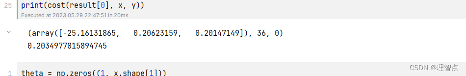
theta = np.zeros((x.shape[1], 1))def cost(theta_param, x_param, y_param):#这里为什么要reshape一下呢？因为cost函数在被fmin_tnc调用的时候，传进来的theta_param会变成一个一维数组，然后就会报错tnc: gradient must have shape (len(x0),)theta_param = np.reshape(theta_param, (x.shape[1], 1))tmp = h_fun(x_param, theta_param)return -(np.sum(np.multiply(y_param, np.log(tmp)) + np.multiply(1 - y_param, np.log(1 - tmp)))) / len(x_param)def gradient(theta_param, x_param, y_param):# 这里reshape的原因同上theta_param = np.reshape(theta_param, (x.shape[1], 1))return (x_param.T @ (h_fun(x_param, theta_param) - y_param)) / len(x_param)result = opt.fmin_tnc(func=cost, x0=theta, fprime=gradient, args=(x, y))print(result)
print(cost(result[0], x, y))

结果

在这里插入图片描述

思路

首先，解答几个可能的问题

为什么要重新定义一个cost代价函数，而不是用之前定义过得j_fun呢？

因为opt.fmin_tnc中对于代价函数的定义是这样的

func : callable ``func(x, *args)``Function to minimize.  Must do one of:1. Return f and g, where f is the value of the function and g itsgradient (a list of floats).2. Return the function value but supply gradient functionseparately as `fprime`.3. Return the function value and set ``approx_grad=True``.If the function returns None, the minimizationis aborted.

我们需要把theta参数放在第一个位置中，并且函数返回的类型有两种选择
第一种是返回代价函数的值和其梯度
第二种是只返回代价函数的值，然后传入fprime参数，fprime函数是梯度计算函数

因此我选择了重新开了一个函数用于计算代价

为什么要对theta_param变量进行reshape操作？theta_param = np.reshape(theta_param, (x.shape[1], 1))

我们的待学习参数x0=theta传入进去之后，会被转化成一个一维数组，然后再去调用我们的cost和gradien函数，因此如果不对theta_param进行reshape操作的话，我们的函数无法正确的运行

会报错 tnc: gradient must have shape (len(x0),)

而且这一点很难排查，我搜了好多遍资料都只说了是gradient函数返回值的问题，但其实真正的问题是因为我们函数中将theta当做一个矩阵来处理，但是在经过调用之后theta_param变成了一个一维数组。

如果你也遇到了这个问题，并且想要进行排查的话可以在gradient函数中print(theta_param)，我想着能一定程度中亲手解决你的困惑

1.2.4

在这里插入图片描述

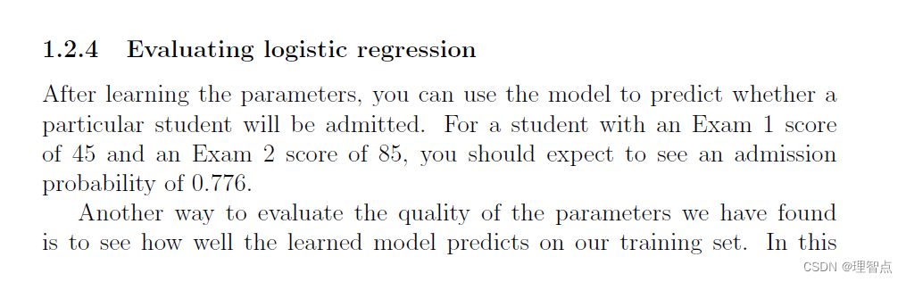
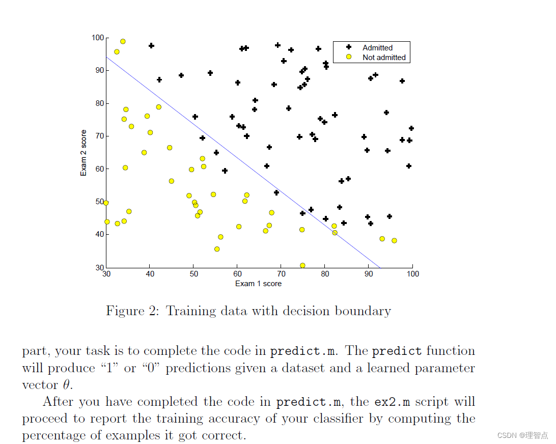
让我们计算一个给定成绩的通过率，并且让我们画出决策边界

代码

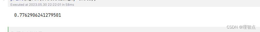
预测

# 保存学习参数
theta = result[0]
# 生成待预测成绩
evaluation_x = np.array([1, 45, 85])
# 查看当前模型该成绩的通过率
print(h_fun(evaluation_x, theta))

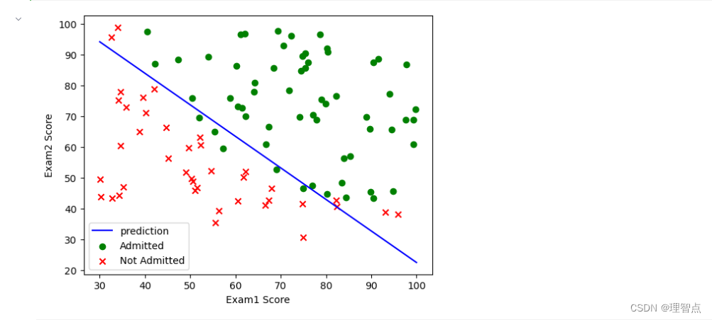
绘图

# 画出决策边界
# 为什么决策边界这样子计算呢，因为决策边界就是J(x,theta) = 0 的时候，移项就成了plt_y,具体的解析可以看下面的 '思路'
plt_x = np.linspace(30, 100, 100)
plt_y = (theta[0] + theta[1] * plt_x) / -(theta[2])
plt.plot(plt_x, plt_y, 'b', label='prediction')
# 绘图
plt.scatter(x=positive[exam1_score_label], y=positive[exam2_score_label], marker='o', label='Admitted', color='g')
plt.scatter(x=negative[exam1_score_label], y=negative[exam2_score_label], marker='x', label="Not Admitted", color='r')plt.legend()
plt.xlabel(exam1_score_label)
plt.ylabel(exam2_score_label)
plt.show()

结果

预测
在这里插入图片描述

决策边界图
在这里插入图片描述

思路

这里主要说一下为什么决策边界这样画
因为我们的预测函数h_fun实际上图形是这样的（画的比较丑别介意）
在这里插入图片描述
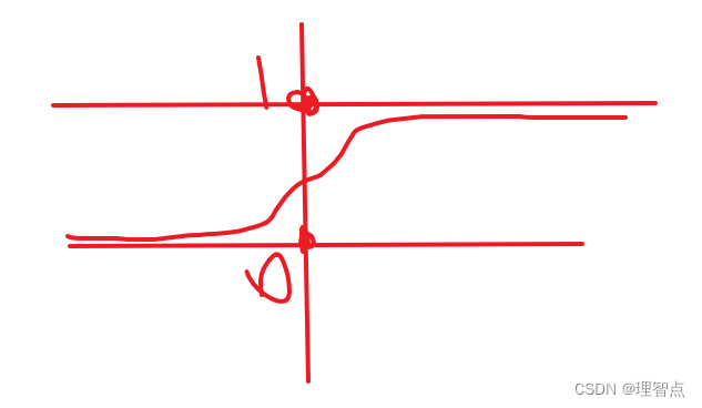
而j_fun又是这个函数

这个函数的特点就是

z的值	g(z)	含义
= 0	等于0.5	决策边界
>0	大于0.5	偏向于1,也就是说positive
<0	小于0.5	偏向于0，也就是negative

源代码

#!/usr/bin/env python
# coding: utf-8# In[2]:import numpy as np
import matplotlib.pyplot as plt
import pandas as pdexam1_score_label = 'Exam1 Score'
exam2_score_label = 'Exam2 Score'
admitted_label = 'Admitted'
# 读取数据
datas = pd.read_csv("./ex2data1.txt", header=None, names=[exam1_score_label, exam2_score_label, admitted_label])
# 获取数据个数
m = len(datas)
#将数据分类用于绘图
positive = datas[datas[admitted_label].isin([1])]
negative = datas[datas[admitted_label].isin([0])]
# 绘图
plt.scatter(x=positive[exam1_score_label], y=positive[exam2_score_label], marker='o', label='Admitted', color='g')
plt.scatter(x=negative[exam1_score_label], y=negative[exam2_score_label], marker='x', label="Not Admitted", color='r')plt.legend()
plt.xlabel(exam1_score_label)
plt.ylabel(exam2_score_label)
plt.show()# In[3]:# 处理数据# 这个判断防止写脚本的时候多次插入bias行
if 'bias' not in datas.columns:datas.insert(0, 'bias', 1)
datas.head()
x = np.matrix(datas.iloc[:, 0:3])
y = np.matrix(datas.iloc[:, 3:4])
# theta = np.matrix(np.zeros(x.shape[1]))
theta = np.zeros((x.shape[1], 1))# In[4]:# 定义预测函数
def h_fun(x_param, theta_param):return sigmoid(x_param @ theta_param)# 定义sigmoid函数
def sigmoid(z_param):return 1 / (1 + np.exp(-z_param))# 定义损失函数
def j_fun(theta_param, x_param, y_param):tmp = h_fun(x_param, theta_param)# print(-np.sum(np.multiply(y_param, np.log(tmp)) + np.multiply(1 - y_param, np.log(1 - tmp))) / len(x_param))return -(np.sum(np.multiply(y_param, np.log(tmp)) + np.multiply(1 - y_param, np.log(1 - tmp)))) / len(x_param)# 查看默认theta的损失函数值
last_cost = j_fun(theta, x, y)
print(last_cost)# In[5]:# 这里对theta重定义是为了方便调试脚本
theta = np.zeros((x.shape[1], 1))# 自己写梯度下降
def gradient_descent(alpha, iteration, train_x, train_y, train_theta):for i in range(iteration):tmp = h_fun(train_x, train_theta)train_theta = train_theta - (alpha / m) * (train_x.T @ (tmp - train_y))return train_theta#手动进行梯度下降
# theta = gradient_descent(0.004, 300000, x, y, theta)
# print(j_fun(theta, x, y))# In[10]:# 使用 fminunc 函数来代替自己实现梯度下降
# 由于我们使用的是Python,所以我们使用scipy.optimize库来实现
import scipy.optimize as opt#重新赋值theta方便调试
theta = np.zeros((x.shape[1], 1))def cost(theta_param, x_param, y_param):#这里为什么要reshape一下呢？因为cost函数在被fmin_tnc调用的时候，传进来的theta_param会变成一个一维数组，然后就会报错tnc: gradient must have shape (len(x0),)theta_param = np.reshape(theta_param, (x.shape[1], 1))tmp = h_fun(x_param, theta_param)return -(np.sum(np.multiply(y_param, np.log(tmp)) + np.multiply(1 - y_param, np.log(1 - tmp)))) / len(x_param)def gradient(theta_param, x_param, y_param):# 这里reshape的原因同上theta_param = np.reshape(theta_param, (x.shape[1], 1))return (x_param.T @ (h_fun(x_param, theta_param) - y_param)) / len(x_param)result = opt.fmin_tnc(func=cost, x0=theta, fprime=gradient, args=(x, y))print(cost(theta,x,y))
print(result)
print(cost(result[0], x, y))# In[7]:# 保存学习参数
theta = result[0]
# 生成待预测成绩
evaluation_x = np.array([1, 45, 85])
# 查看当前模型该成绩的通过率
print(h_fun(evaluation_x, theta))# In[8]:# 画出决策边界
# 为什么决策边界这样子计算呢，因为决策边界就是J(x,theta) = 0 的时候，移项就成了plt_y,具体的解析可以看下面的 '思路'
plt_x = np.linspace(30, 100, 100)
plt_y = (theta[0] + theta[1] * plt_x) / -(theta[2])
plt.plot(plt_x, plt_y, 'b', label='prediction')
# 绘图
plt.scatter(x=positive[exam1_score_label], y=positive[exam2_score_label], marker='o', label='Admitted', color='g')
plt.scatter(x=negative[exam1_score_label], y=negative[exam2_score_label], marker='x', label="Not Admitted", color='r')plt.legend()
plt.xlabel(exam1_score_label)
plt.ylabel(exam2_score_label)
plt.show()

第二题

2.1 数据可视化

在这里插入图片描述

代码

import numpy as np
import matplotlib.pyplot as plt
import pandas as pdmicrochip_test1_label = "Microchip Test 1"
microchip_test2_label = "MicroChip Test 2"
admitted_label = "Admitted"#读取数据
datas = pd.read_csv("./ex2data2.txt", header=None, names=[microchip_test1_label, microchip_test2_label, admitted_label])
# 获取数据个数
m = len(datas)
# 对数据进行分组
positive = datas.groupby(admitted_label).get_group(1)
negative = datas.groupby(admitted_label).get_group(0)# 绘图
plt.scatter(x=positive[microchip_test1_label], y=positive[microchip_test2_label], marker='o', c='g', label='Admitted')
plt.scatter(x=negative[microchip_test1_label], y=negative[microchip_test2_label], marker='x', c='r',label='Not Admitted')
plt.legend()
plt.xlabel(microchip_test1_label)
plt.ylabel(microchip_test2_label)
plt.show()

结果

在这里插入图片描述

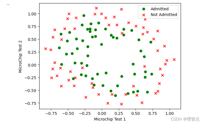
讲解

没啥好说的，按照第一题的思路我们直接复用即可

2.2 特征值映射

在这里插入图片描述

代码

x = datas.iloc[:, 0:2]
y = np.array(datas.iloc[:, 2:3])# feature mapping 特征值映射
def feature_mapping(x_param):degree = 6x1 = x_param.iloc[:, 0]x2 = x_param.iloc[:, 1]# 创建一个空的对象用于返回result = pd.DataFrame()for i in range(1, degree + 1):for j in range(0, i + 1):result['F' + str(i) + str(j)] = np.power(x1, i - j) * np.power(x2, j)# 插入 bias 列result.insert(0, 'bias', 1)return resultx = feature_mapping(x)
x = np.array(x)

讲解

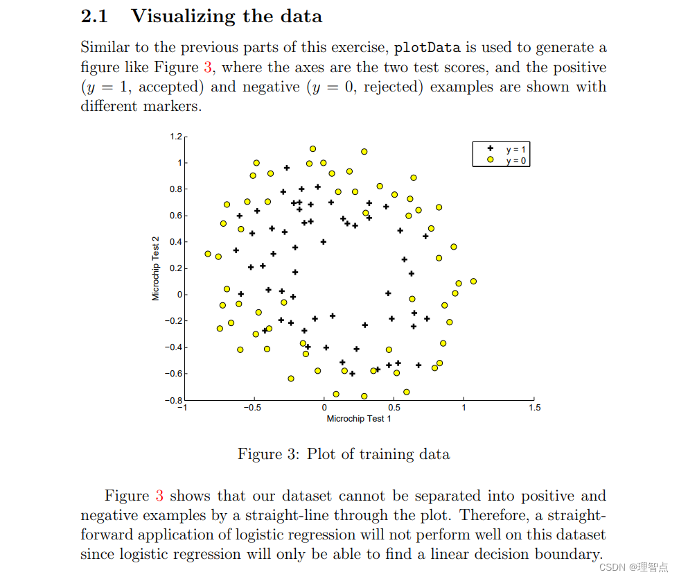
为什么要进行特征值映射

首先，从数据可视化后的图像中我们可以看到决策边界大概是一个比较复杂的图像，
不是普普通通的一元一次或者二元二次函数可以进行拟合的
因此，我们可以进行特征值映射，增加我们的特征值数量，来方便我们进行更高层次的拟合
也就是更加复杂函数的拟合

2.3 损失函数及其梯度

在这里插入图片描述

代码

# 定义几个函数# 定义 sigmoid 函数
def sigmoid(z_param):return 1 / (1 + np.exp(-z_param))# 定义预测函数
def h_fun(theta_param, x_param):return sigmoid(x_param @ theta_param)# 定义损失函数
def cost(theta_param, x_param, y_param, l):theta_param = np.reshape(theta_param, (x_param.shape[1], 1))tmp = h_fun(theta_param, x_param)tmp_1 = -np.multiply(y_param, np.log(tmp))tmp_2 = -np.multiply(1 - y_param, np.log(1 - tmp))return np.sum(tmp_1 + tmp_2) / m + l / (2 * m) * np.sum(np.power(theta_param, 2))# 定义梯度函数
def gradient(theta_param, x_param, y_param, l):theta_param = np.reshape(theta_param, (x_param.shape[1], 1))cpy_theta_param = theta_param.copy()tmp = h_fun(theta_param, x_param)theta_param = (x_param.T @ (tmp - y_param)) / mtheta_param[1:, :] += l / m * cpy_theta_param[1:, :]return theta_param

讲解

有了之前的经验，这几个函数具体的定义我就不讲了，其中注意一点就是梯度函数中的theta_param变量的更新，我为什么会这样写呢？
因为我这里在更新前提前保存了一份 theta_param 作为cpy_theta_param
同时因为带有lambda项的损失函数在计算式当j = 0 时更新策略有所不同，所以我才用了这样的方式来进行更新。

2.3.1 使用fuminc进行参数拟合

在这里插入图片描述

代码

# 使用 fminunc
import scipy.optimize as opttheta = np.zeros((x.shape[1],))result = opt.fmin_tnc(func=cost, x0=theta, fprime=gradient, args=(x, y, 1))theta = result[0]
print(theta)

讲解

没啥好说的
跑就完事了，需要注意的点在第一题那里都说过了

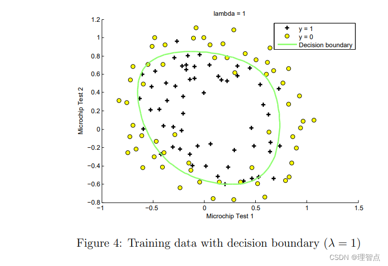
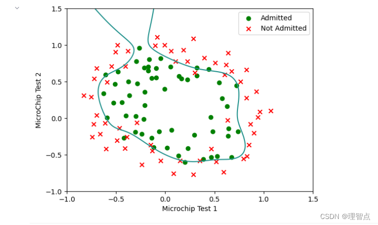
2.4 绘制决策边界

代码

# 绘图 (这里的绘图我是抄别人的，因为我对 numpy 和 matplotlib这几个库不是很了解，所以我就不发表我的拙见了)
# 准备用于绘制决策边界的数据# 特征工程
def featureMapping(x1, x2, degree):data = {}for i in np.arange(degree + 1):for j in np.arange(i + 1):data["F{}{}".format(i - j, j)] = np.power(x1, i - j) * np.power(x2, j)passreturn pd.DataFrame(data)plt_x = np.linspace(-1, 1.5, 150)
plt_xx, plt_yy = np.meshgrid(plt_x, plt_x)
z = np.array(featureMapping(plt_xx.ravel(), plt_yy.ravel(), 6))
z = z @ theta
z = z.reshape(plt_xx.shape)# 绘图
plt.scatter(x=positive[microchip_test1_label], y=positive[microchip_test2_label], marker='o', c='g', label='Admitted')
plt.scatter(x=negative[microchip_test1_label], y=negative[microchip_test2_label], marker='x', c='r',label='Not Admitted')
plt.legend()
plt.xlabel(microchip_test1_label)
plt.ylabel(microchip_test2_label)
plt.contour(plt_xx, plt_yy, z, 0)
plt.show()

结果

在这里插入图片描述

讲解

因为我不会很好的使用py的几个库，所以这里的绘图我是抄别人的，我就不发表自己的拙见了。

2.5 可选练习（尝试不同的Lambda值）

在这里插入图片描述

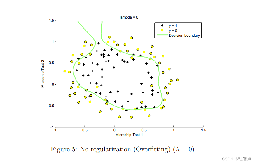
讲解

只要把代码中的

result = opt.fmin_tnc(func=cost, x0=theta, fprime=gradient, args=(x, y, 1))

最后一个1 改成 0 即可
最后画出来的图片（过拟合曲线）为

在这里插入图片描述

源代码

#!/usr/bin/env python
# coding: utf-8# In[11]:import numpy as np
import matplotlib.pyplot as plt
import pandas as pdmicrochip_test1_label = "Microchip Test 1"
microchip_test2_label = "MicroChip Test 2"
admitted_label = "Admitted"#读取数据
datas = pd.read_csv("./ex2data2.txt", header=None, names=[microchip_test1_label, microchip_test2_label, admitted_label])
# 获取数据个数
m = len(datas)
# 对数据进行分组
positive = datas.groupby(admitted_label).get_group(1)
negative = datas.groupby(admitted_label).get_group(0)# 绘图
plt.scatter(x=positive[microchip_test1_label], y=positive[microchip_test2_label], marker='o', c='g', label='Admitted')
plt.scatter(x=negative[microchip_test1_label], y=negative[microchip_test2_label], marker='x', c='r',label='Not Admitted')
plt.legend()
plt.xlabel(microchip_test1_label)
plt.ylabel(microchip_test2_label)
plt.show()# In[12]:x = datas.iloc[:, 0:2]
y = np.array(datas.iloc[:, 2:3])# feature mapping 特征值映射
def feature_mapping(x_param):degree = 6x1 = x_param.iloc[:, 0]x2 = x_param.iloc[:, 1]# 创建一个空的对象用于返回result = pd.DataFrame()for i in range(1, degree + 1):for j in range(0, i + 1):result['F' + str(i) + str(j)] = np.power(x1, i - j) * np.power(x2, j)# 插入 bias 列result.insert(0, 'bias', 1)return resultx = feature_mapping(x)
x = np.array(x)# In[13]:# 定义几个函数# 定义 sigmoid 函数
def sigmoid(z_param):return 1 / (1 + np.exp(-z_param))# 定义预测函数
def h_fun(theta_param, x_param):return sigmoid(x_param @ theta_param)# 定义损失函数
def cost(theta_param, x_param, y_param, l):theta_param = np.reshape(theta_param, (x_param.shape[1], 1))tmp = h_fun(theta_param, x_param)tmp_1 = -np.multiply(y_param, np.log(tmp))tmp_2 = -np.multiply(1 - y_param, np.log(1 - tmp))return np.sum(tmp_1 + tmp_2) / m + l / (2 * m) * np.sum(np.power(theta_param, 2))# 定义梯度函数
def gradient(theta_param, x_param, y_param, l):theta_param = np.reshape(theta_param, (x_param.shape[1], 1))cpy_theta_param = theta_param.copy()tmp = h_fun(theta_param, x_param)theta_param = (x_param.T @ (tmp - y_param)) / mtheta_param[1:, :] += l / m * cpy_theta_param[1:, :]return theta_param# In[14]:# 使用 fminunc
import scipy.optimize as opttheta = np.zeros((x.shape[1],))result = opt.fmin_tnc(func=cost, x0=theta, fprime=gradient, args=(x, y, 0))theta = result[0]
print(theta)# In[15]:# 绘图 (这里的绘图我是抄别人的，因为我对 numpy 和 matplotlib这几个库不是很了解，所以我就不发表我的拙见了)
# 准备用于绘制决策边界的数据# 特征工程
def featureMapping(x1, x2, degree):data = {}for i in np.arange(degree + 1):for j in np.arange(i + 1):data["F{}{}".format(i - j, j)] = np.power(x1, i - j) * np.power(x2, j)passreturn pd.DataFrame(data)plt_x = np.linspace(-1, 1.5, 150)
plt_xx, plt_yy = np.meshgrid(plt_x, plt_x)
z = np.array(featureMapping(plt_xx.ravel(), plt_yy.ravel(), 6))
z = z @ theta
z = z.reshape(plt_xx.shape)# 绘图
plt.scatter(x=positive[microchip_test1_label], y=positive[microchip_test2_label], marker='o', c='g', label='Admitted')
plt.scatter(x=negative[microchip_test1_label], y=negative[microchip_test2_label], marker='x', c='r',label='Not Admitted')
plt.legend()
plt.xlabel(microchip_test1_label)
plt.ylabel(microchip_test2_label)
plt.contour(plt_xx, plt_yy, z, 0)
plt.show()