Hands on RL 之 Proximal Policy Optimization (PPO)

1. 回顾Policy Gradient和TRPO

​ 首先回顾一下Policy Gradient （PG）的方法，在策略梯度方法PG中，我们使用参数化的神经网络（Neural Network，NN）$\pi (a|s;\theta )$或${\pi }_{\theta }(a|s)$来表示策略网络，则我们需要优化的目标函数可以写作
$$\text{PG:}{L}^{PG}(\theta )={\hat{\mathbb{E}}}_t[\log {\pi }_{\theta }(a_t|s_t){\hat{A}}_t]$$
其中${\hat{A}}_t$是对优势函数（Advantage Function）的估计，这表明已经将状态价值作为baseline $b(S)$了，$L^{PG}$表示的是policy gradient。

​ 然后再回顾一下Trust Region Policy Optimization （TRPO）的方法，在TRPO中引入了KL散度（Kullback-Leibler Divergence）的概念，KL散度是用于描述我们用概率分布Q来估计真是分布P的编码损失。

KL散度的定义如下

​ 假设对随机变量$\xi$，存在两个概率分布P和Q，其中P是真实的概率分布，Q是较容易获得的概率分布。如果$\xi$是离散的随机变量，那么定义从P到Qd KL散度为
$${\mathbb{D}}_{KL}(P,Q)=\sum _{i}P(i)\ln (\frac{P(i)}{Q(i)})$$
如果$\xi$是连续变量，则定义从P到Q的KL散度为
$${\mathbb{D}}_{KL}(P,Q)={\int }_{-\infty }^{\infty }p(x)\ln (\frac{p(x)}{q(x)})dx$$
​ 在TRPO中待优化的目标函数即为
$$\text{TRPO:}\{\begin{array}{rl}\underset{\theta }{\max }& L^{TRPO}(\theta )={\hat{\mathbb{E}}}_t\left[\frac{{\pi }_{\theta }(a_t|s_t)}{{\pi }_{{\theta }_{\text{old}}}(a_t|s_t)}{\hat{A}}_t\right]\\ \text{subject to}& {\hat{\mathbb{E}}}_t\left[{\mathbb{D}}_{KL}\right({\pi }_{{\theta }_{\text{old}}}(\cdot |s_t),{\pi }_{\theta }(\cdot |s_t)\left)\right]\le \delta \end{array}$$
其中$L^{TRPO}$表示 trust region policy optimization，${\theta }_{\text{old}}$表示更新前的网络参数。

2. PPO (Clip)

​ 在介绍之前先定义几个符号，用$r_t(\theta )$来表示概率比，即$r_t(\theta )=\frac{{\pi }_{\theta }(a_t|s_t)}{{\pi }_{{\theta }_{\text{old}}}(a_t|s_t)}$，那么则有$r_t({\theta }_{\text{old}})=1$，所以在TRPO中待优化的目标函数就变成了
$$L^{TRPO}={\hat{\mathbb{E}}}_t\left[\frac{{\pi }_{\theta }(a_t|s_t)}{{\pi }_{{\theta }_{\text{old}}}(a_t|s_t)}{\hat{A}}_t\right]={\hat{\mathbb{E}}}_t[r_t(\theta ){\hat{A}}_t]$$
PPO clip版本就是在TRPO的基础上增加了截断（clip）的操作，截断即是将概率比限制在一定的范围之内，即$r_t(\theta )\in [1-ϵ,1+ϵ]$，其中$ϵ$是指定范围的超参数表示截断的范围，一般设置$ϵ=0.2$。修改后的替代目标（surrogate objective）可以表示为
$$\text{PPO-clip:}{L}^{CLIP}(\theta )={\hat{\mathbb{E}}}_t[\min (r_t(\theta ){\hat{A}}_t,\text{clip}(r_t(\theta ),1-ϵ,1+ϵ){\hat{A}}_t)]$$
其中$L^{CLIP}$表示PPO-clip，截断操作是$\text{clip}(r_t(\theta ),1-ϵ,1+ϵ)$的操作为$\max (\min (r_t(\theta ),1+ϵ),1-ϵ)$，即让$r_t(\theta )\in [1-ϵ,1+ϵ]$。

clip操作的解释如下所示

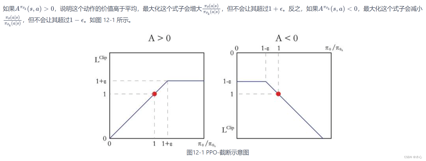
3. PPO(Penalty)

​ PPO penalty版本的改进非常简单，就是在TRPO的基础上，将TRPO中的约束条件作为惩罚项（penalty）加入到目标函数中，并且使用一个自适应的学习率来更新惩罚项。数学的表示即为

$$\text{PPO-penalty:}{L}^{KLPEN}(\theta )={\hat{\mathbb{E}}}_t[\frac{{\pi }_{\theta }(a_t|s_t)}{{\pi }_{{\theta }_{\text{old}}}(a_t|s_t)}{\hat{A}}_t-\beta {\mathbb{D}}_{KL}({\pi }_{{\theta }_{\text{old}}}(\cdot |s_t),{\pi }_{\theta }(\cdot |s_t)\left)\right]$$

其中$\beta$按照以下方式进行更新

$$\begin{array}{rl}d& ={\hat{\mathbb{E}}}_t[{\mathbb{D}}_{KL}({\pi }_{{\theta }_{\text{old}}}(\cdot |s_t),{\pi }_{\theta }(\cdot |s_t))]\\ \text{If }d& <d_{targ}/1.5,\beta \leftarrow \beta /2\\ \text{If }d& >d_{targ}\times 1.5,\beta \leftarrow \beta \times 2\end{array}$$

原论文中指出，经过大量实验表明，PPO-clip的效果总是要优于PPO-penalty。

4. PPO中Advantage Function的计算

Advantage function优势函数的定义是

$${\hat{A}}_t=Q(s_t,a_t)-V(s_t)$$

当我们使用类似n-step Sarsa的方式来估计$Q(s_t,a_t)$时，那么优势函数就变为

$${\hat{A}}_t=r_t+\gamma r_{t+1}+\cdots +{\gamma }^{T-t+1}{r}_{T-1}+{\gamma }^{T-t}V(s_T)-V(s_t)$$

为了方便使用，我们可以将上式再写成truncated fashion截断的形式

$$\begin{array}{rl}& {\hat{A}}_t={\delta }_t+(\gamma \lambda ){\delta }_{t+1}+\cdots +(\gamma \lambda {)}^{T-t+1}{\delta }_{T-1}\\ \text{where }& {\delta }_t=r_t+\gamma V(s_{t+1})-V(s_t)\end{array}$$

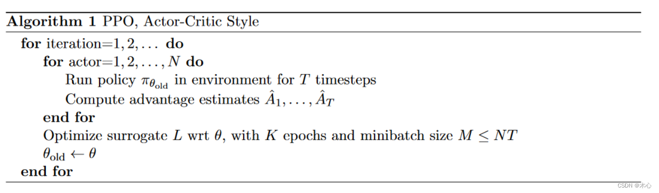
Pesudocode

5.实现 PPO-Clip

import torch
import torch.nn as nn
import torch.nn.functional as F
from tqdm import tqdm
import gym
import numpy as np
import matplotlib.pyplot as plt# Policy Network
class PolicyNet(nn.Module):def __init__(self, state_dim, hidden_dim, action_dim):super(PolicyNet, self).__init__()self.fc1 = nn.Linear(in_features=state_dim, out_features=hidden_dim)self.fc2 = nn.Linear(in_features=hidden_dim, out_features=action_dim)def forward(self, observation):x = F.relu(self.fc1(observation))x = F.softmax(self.fc2(x), dim=1)return x# State Value Network
class ValueNet(nn.Module):def __init__(self, state_dim, hidden_dim):super(ValueNet, self).__init__()self.fc1 = nn.Linear(in_features=state_dim, out_features=hidden_dim)self.fc2 = nn.Linear(in_features=hidden_dim, out_features=1)def forward(self, observation):x = F.relu(self.fc1(observation))return self.fc2(x)# PPO Clip Algorithm
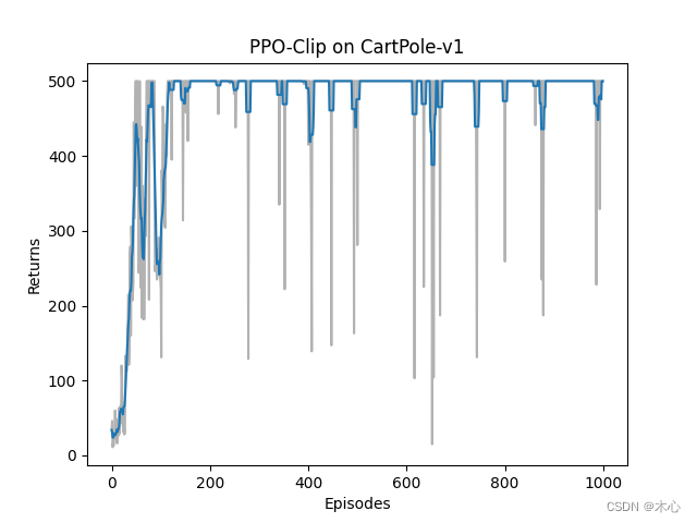
class PPO_clip():def __init__(self, state_dim, hidden_dim, action_dim, actor_lr, critic_lr, lmbda, epochs, eps, gamma, device):self.actor = PolicyNet(state_dim, hidden_dim, action_dim).to(device)self.critic = ValueNet(state_dim, hidden_dim).to(device)self.actor_optimizer = torch.optim.Adam(self.actor.parameters(), lr=actor_lr)self.critic_optimizer = torch.optim.Adam(self.critic.parameters(), lr=critic_lr)self.device = deviceself.lmbda = lmbdaself.gamma = gammaself.epochs = epochs    # 一条序列的数据用来训练的轮数self.eps = eps          # PPO中截断范围的参数def calculate_advantage(self, td_delta):# compute advantage over td_deltatd_delta = td_delta.detach().numpy()temp = 0advantage_list = []for td in td_delta[::-1]:temp = temp * self.gamma * self.lmbda + tdadvantage_list.append(temp)advantage = torch.tensor(np.array(advantage_list[::-1]), dtype=torch.float)return advantage.to(self.device)def choose_action(self, state):state = torch.tensor([state], dtype=torch.float).to(self.device)probs = self.actor(state)action_dist = torch.distributions.Categorical(probs)action = action_dist.sample().item()return actiondef learn(self, transition_dict):states = torch.tensor(transition_dict['states'], dtype=torch.float).to(self.device)actions = torch.tensor(transition_dict['actions'], dtype=torch.int64).view(-1,1).to(self.device)rewards = torch.tensor(transition_dict['rewards'], dtype=torch.float).view(-1,1).to(self.device)next_states = torch.tensor(transition_dict['next_states'], dtype=torch.float).to(self.device)dones = torch.tensor(transition_dict['dones'], dtype=torch.float).view(-1,1).to(self.device)td_target = rewards + self.gamma * self.critic(next_states) * (1-dones)td_delta = td_target - self.critic(states)advantage = self.calculate_advantage(td_delta.cpu())old_log_probs = torch.log(self.actor(states).gather(dim=1, index=actions)).detach()for _ in range(self.epochs):log_probs = torch.log(self.actor(states).gather(dim=1, index=actions))ratio = torch.exp(log_probs - old_log_probs)surr1 = ratio * advantagesurr2 = torch.clamp(ratio, 1-self.eps, 1+self.eps) * advantageactor_loss = torch.mean(-torch.min(surr1, surr2))critic_loss = torch.mean(F.mse_loss(td_target.detach(), self.critic(states)))self.actor_optimizer.zero_grad()self.critic_optimizer.zero_grad()actor_loss.backward()critic_loss.backward()self.actor_optimizer.step()self.critic_optimizer.step()def train_on_policy_agent(env, agent, num_episodes, render, seed_number):return_list = []for i in range(10):with tqdm(total=int(num_episodes/10), desc="Iteration:%d"%(i+1)) as pbar:for i_episode in range(int(num_episodes/10)):episode_return = 0done = Falsetransition_dict = {'states': [],'actions': [],'next_states': [],'rewards': [],'dones': []}observation, _ = env.reset(seed=seed_number)while not done:if render:env.render()action = agent.choose_action(observation)observation_, reward, terminated, truncated, _ = env.step(action)done = terminated or truncated# save one episode experience into a dicttransition_dict['states'].append(observation)transition_dict['actions'].append(action)transition_dict['rewards'].append(reward)transition_dict['next_states'].append(observation_)transition_dict['dones'].append(done)# swap stateobservation = observation_# compute one episode returnepisode_return += rewardreturn_list.append(episode_return)# agent learningagent.learn(transition_dict)if((i_episode + 1) % 10 == 0):pbar.set_postfix({'episode': '%d'%(num_episodes / 10 * i + i_episode + 1),'return': '%.3f'%(np.mean(return_list[-10:]))})pbar.update(1)env.close()return return_listdef moving_average(a, window_size):cumulative_sum = np.cumsum(np.insert(a, 0, 0)) middle = (cumulative_sum[window_size:] - cumulative_sum[:-window_size]) / window_sizer = np.arange(1, window_size-1, 2)begin = np.cumsum(a[:window_size-1])[::2] / rend = (np.cumsum(a[:-window_size:-1])[::2] / r)[::-1]return np.concatenate((begin, middle, end))def plot_curve(return_list, mv_return, algorithm_name, env_name):episodes_list = list(range(len(return_list)))plt.plot(episodes_list, return_list, c='gray', alpha=0.6)plt.plot(episodes_list, mv_return)plt.xlabel('Episodes')plt.ylabel('Returns')plt.title('{} on {}'.format(algorithm_name, env_name))plt.show()if __name__ == "__main__":# reproducibleseed_number = 0np.random.seed(seed_number)torch.manual_seed(seed_number)num_episodes = 1000     # episodes lengthhidden_dim = 256        # hidden layers dimensiongamma = 0.98            # discounted ratelmbda = 0.95            # coefficient for computing advantage epochs = 10             # update parameters intervaleps = 0.2               # clip coefficientactor_lr = 1e-3         # lr of actorcritic_lr = 1e-2        # lr of criticdevice = torch.device('cuda' if torch.cuda.is_available() else 'gpu')env_name = 'CartPole-v1'render = Falseif render:env = gym.make(id=env_name, render_mode='human')else:env = gym.make(id=env_name)state_dim = env.observation_space.shape[0]action_dim = env.action_space.nagent = PPO_clip(state_dim, hidden_dim, action_dim, actor_lr, critic_lr, lmbda, epochs, eps, gamma, device)return_list = train_on_policy_agent(env, agent, num_episodes, render, seed_number)mv_return = moving_average(return_list, 9)plot_curve(return_list, mv_return, 'PPO-Clip', env_name)

最后的训练回报（return）曲线如下

Reference

Tutorial: Hands on RL

Paper: Proximal Policy Optimization Algorithm