【图像分割】图像检测（分割、特征提取）、各种特征（面积等）的测量和过滤（Matlab代码实现）

💥💥💞💞欢迎来到本博客❤️❤️💥💥

🏆博主优势：🌞🌞🌞博客内容尽量做到思维缜密，逻辑清晰，为了方便读者。

⛳️座右铭：行百里者，半于九十。

📋📋📋本文目录如下：🎁🎁🎁

目录

💥1 概述

📚2 运行结果

🎉3 参考文献

🌈4 Matlab代码实现

💥1 概述

【图像分割】图像检测（分割、特征提取）、各种特征（面积等）的测量和过滤

本文提供了一个适合初学者的教程，旨在演示图像检测（分割、特征提取）以及各种特征（如面积）的测量和过滤（只提取某些对象）。

首先，该教程介绍了如何找到图像中的所有对象（硬币），然后根据指定的直径过滤结果，筛选出特定直径的对象。通过一个简单的示例，展示了阈值处理、标记和区域属性的基本概念。

对于那些刚开始接触 MATLAB 图像处理功能的同学来说，这个教程是一个很好的起点。在他们深入学习更复杂的算法之前，可以通过这个教程加深对基本概念和技术的理解。

为了完成这个教程，需要安装图像处理工具箱，因为它演示了该工具箱提供的某些功能。同时，教程使用了工具箱自带的一个名为“硬币”的示例图像作为演示对象。

该教程的优点在于，它提供了一种直观和实用的方法，帮助初学者理解如何使用 MATLAB 对图像进行处理和分析。通过学习如何进行图像分割、特征提取和过滤，读者将受益于这些基本概念，并能够应用它们解决更为复杂的图像处理问题。这个教程对于那些有兴趣进一步探索图像处理领域的学生、研究人员和工程师来说，都是一个很好的起点。

📚2 运行结果

部分代码：

% Read in a standard MATLAB demo image of coins (US nickles and dimes, which are 5 cent and 10 cent coins).  This image ships with MATLAB.
baseFileName = 'coins.png';
folder = fileparts(which(baseFileName)); % Determine where demo folder is (works with all versions).
fullFileName = fullfile(folder, baseFileName);
fprintf('Full File Name = "%s".\n', fullFileName);
if ~exist(fullFileName, 'file')% It doesn't exist in the current folder.% Look on the search path.if ~exist(baseFileName, 'file')% It doesn't exist on the search path either.% Alert user that we can't find the image.warningMessage = sprintf('Error: the input image file\n%s\nwas not found.\nClick OK to exit the demo.', fullFileName);uiwait(warndlg(warningMessage));fprintf(1, 'Finished running BlobsDemo.m.\n');return;end% Found it on the search path.  Construct the file name.fullFileName = baseFileName; % Note: don't prepend the folder.
end
% If we get here, we should have found the image file.
originalImage = imread(fullFileName);
% Check to make sure that it is grayscale, just in case the user substituted their own image.
[rows, columns, numberOfColorChannels] = size(originalImage);
if numberOfColorChannels > 1promptMessage = sprintf('Your image file has %d color channels.\nThis demo was designed for grayscale images.\nDo you want me to convert it to grayscale for you so you can continue?', numberOfColorChannels);button = questdlg(promptMessage, 'Continue', 'Convert and Continue', 'Cancel', 'Convert and Continue');if strcmp(button, 'Cancel')fprintf(1, 'Finished running BlobsDemo.m.\n');return;end% Do the conversion using standard book formulaoriginalImage = rgb2gray(originalImage);
end% Display the grayscale image.
subplot(3, 3, 1);
imshow(originalImage);
% Maximize the figure window.
hFig1 = gcf;
hFig1.Units = 'normalized';
hFig1.WindowState = 'maximized'; % Go to full screen.
hFig1.NumberTitle = 'off'; % Get rid of "Figure 1"
hFig1.Name = 'Demo by Image Analyst'; % Put this into title bar.
% Force it to display RIGHT NOW (otherwise it might not display until it's all done, unless you've stopped at a breakpoint.)
drawnow;
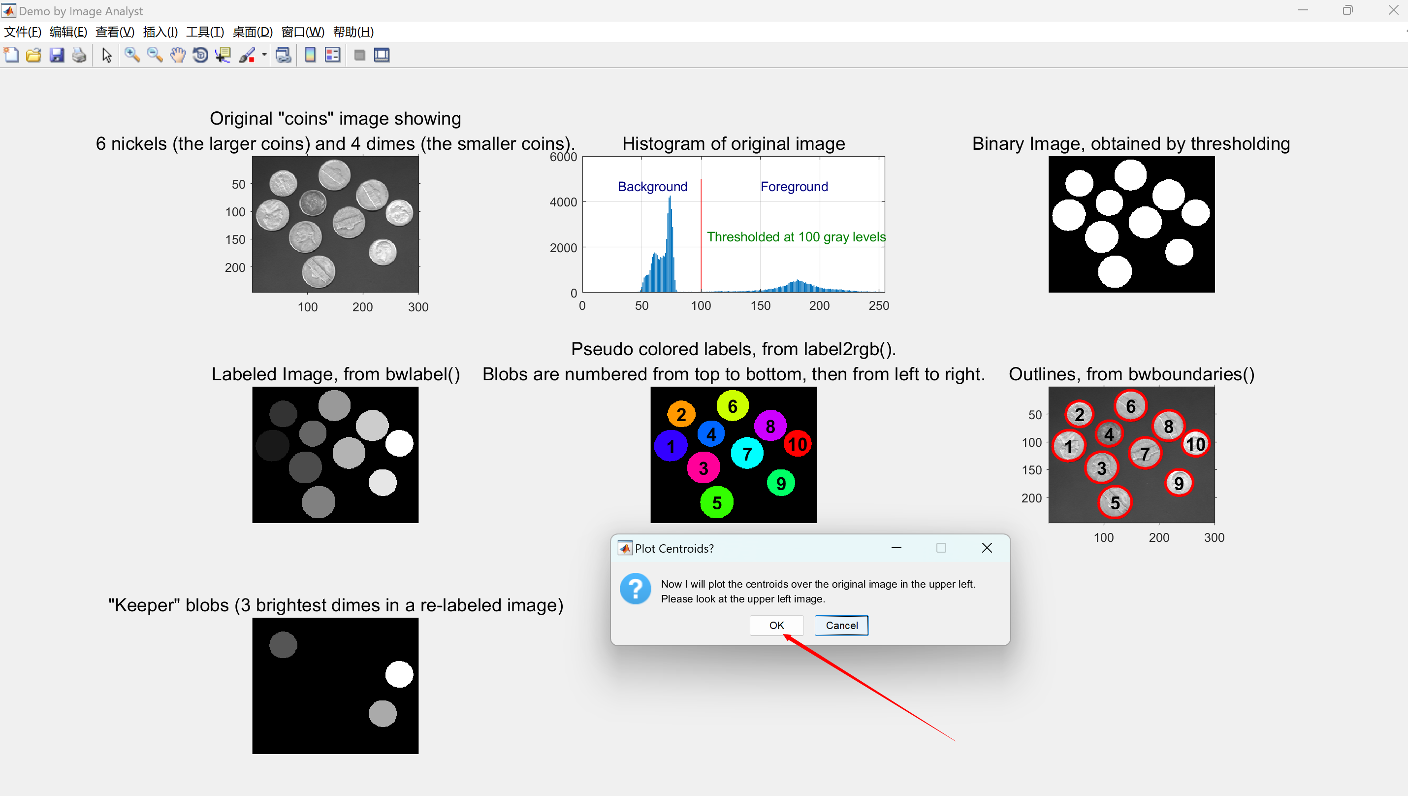
caption = sprintf('Original "coins" image showing\n6 nickels (the larger coins) and 4 dimes (the smaller coins).');
title(caption, 'FontSize', captionFontSize);
axis('on', 'image'); % Make sure image is not artificially stretched because of screen's aspect ratio.% Just for fun, let's get its histogram and display it.
[pixelCount, grayLevels] = imhist(originalImage);
subplot(3, 3, 2);
bar(pixelCount);
title('Histogram of original image', 'FontSize', captionFontSize);
xlim([0 grayLevels(end)]); % Scale x axis manually.
grid on;%------------------------------------------------------------------------------------------------------------------------------------------------------
% Threshold the image to get a binary image (only 0's and 1's) of class "logical."
% Method #1: using im2bw()
%   normalizedThresholdValue = 0.4; % In range 0 to 1.
%   thresholdValue = normalizedThresholdValue * max(max(originalImage)); % Gray Levels.
%   binaryImage = im2bw(originalImage, normalizedThresholdValue);       % One way to threshold to binary
% Method #2: using a logical operation.
thresholdValue = 100;
binaryImage = originalImage > thresholdValue; % Bright objects will be chosen if you use >.
% ========== IMPORTANT OPTION ============================================================
% Use < if you want to find dark objects instead of bright objects.
%   binaryImage = originalImage < thresholdValue; % Dark objects will be chosen if you use <.% Do a "hole fill" to get rid of any background pixels or "holes" inside the blobs.
binaryImage = imfill(binaryImage, 'holes');% Show the threshold as a vertical red bar on the histogram.
hold on;
maxYValue = ylim;
line([thresholdValue, thresholdValue], maxYValue, 'Color', 'r');
% Place a text label on the bar chart showing the threshold.
annotationText = sprintf('Thresholded at %d gray levels', thresholdValue);
% For text(), the x and y need to be of the data class "double" so let's cast both to double.
text(double(thresholdValue + 5), double(0.5 * maxYValue(2)), annotationText, 'FontSize', 10, 'Color', [0 .5 0]);
text(double(thresholdValue - 70), double(0.94 * maxYValue(2)), 'Background', 'FontSize', 10, 'Color', [0 0 .5]);
text(double(thresholdValue + 50), double(0.94 * maxYValue(2)), 'Foreground', 'FontSize', 10, 'Color', [0 0 .5]);% Display the binary image.
subplot(3, 3, 3);
imshow(binaryImage);
title('Binary Image, obtained by thresholding', 'FontSize', captionFontSize);%------------------------------------------------------------------------------------------------------------------------------------------------------
% Identify individual blobs by seeing which pixels are connected to each other.  This is called "Connected Components Labeling".
% Each group of connected pixels will be given a label, a number, to identify it and distinguish it from the other blobs.
% Do connected components labeling with either bwlabel() or bwconncomp().
[labeledImage, numberOfBlobs] = bwlabel(binaryImage, 8);     % Label each blob so we can make measurements of it
% labeledImage is an integer-valued image where all pixels in the blobs have values of 1, or 2, or 3, or ... etc.
subplot(3, 3, 4);
imshow(labeledImage, []);  % Show the gray scale image.
title('Labeled Image, from bwlabel()', 'FontSize', captionFontSize);
drawnow;% Let's assign each blob a different color to visually show the user the distinct blobs.
coloredLabels = label2rgb (labeledImage, 'hsv', 'k', 'shuffle'); % pseudo random color labels
% coloredLabels is an RGB image.  We could have applied a colormap instead (but only with R2014b and later)
subplot(3, 3, 5);
imshow(coloredLabels);
axis image; % Make sure image is not artificially stretched because of screen's aspect ratio.
caption = sprintf('Pseudo colored labels, from label2rgb().\nBlobs are numbered from top to bottom, then from left to right.');
title(caption, 'FontSize', captionFontSize);%======================================================================================================================================================
% MAIN PART IS RIGHT HERE!!!
% Get all the blob properties.
props = regionprops(labeledImage, originalImage, 'all');
% Or, if you want, you can ask for only a few specific measurements.  This will be faster since we don't have to compute everything.
% props = regionprops(labeledImage, originalImage, 'MeanIntensity', 'Area', 'Perimeter', 'Centroid', 'EquivDiameter');
numberOfBlobs = numel(props); % Will be the same as we got earlier from bwlabel().
%======================================================================================================================================================%------------------------------------------------------------------------------------------------------------------------------------------------------
% PLOT BOUNDARIES.
% Plot the borders of all the coins on the original grayscale image using the coordinates returned by bwboundaries().
% bwboundaries() returns a cell array, where each cell contains the row/column coordinates for an object in the image.
subplot(3, 3, 6);
imshow(originalImage);
title('Outlines, from bwboundaries()', 'FontSize', captionFontSize);
axis('on', 'image'); % Make sure image is not artificially stretched because of screen's aspect ratio.
% Here is where we actually get the boundaries for each blob.
boundaries = bwboundaries(binaryImage); % Note: this is a cell array with several boundaries -- one boundary per cell.
% boundaries is a cell array - one cell for each blob.
% In each cell is an N-by-2 list of coordinates in a (row, column) format.  Note: NOT (x,y).
% Column 1 is rows, or y.    Column 2 is columns, or x.
numberOfBoundaries = size(boundaries, 1); % Count the boundaries so we can use it in our for loop
% Here is where we actually plot the boundaries of each blob in the overlay.
hold on; % Don't let boundaries blow away the displayed image.
for k = 1 : numberOfBoundariesthisBoundary = boundaries{k}; % Get boundary for this specific blob.x = thisBoundary(:,2); % Column 2 is the columns, which is x.y = thisBoundary(:,1); % Column 1 is the rows, which is x.plot(x, y, 'r-', 'LineWidth', 2); % Plot boundary in red.
end
hold off;%------------------------------------------------------------------------------------------------------------------------------------------------------
% Print out the measurements to the command window, and display blob numbers on the image.
textFontSize = 14;	% Used to control size of "blob number" labels put atop the image.
% Print header line in the command window.
fprintf(1,'Blob #      Mean Intensity  Area   Perimeter    Centroid       Diameter\n');
% Extract all the mean diameters into an array.
% The "diameter" is the "Equivalent Circular Diameter", which is the diameter of a circle with the same number of pixels as the blob.
% Enclosing in brackets is a nice trick to concatenate all the values from all the structure fields (every structure in the props structure array).
blobECD = [props.EquivDiameter];
% Loop over all blobs printing their measurements to the command window.
for k = 1 : numberOfBlobs           % Loop through all blobs.% Find the individual measurements of each blob.  They are field of each structure in the props strucutre array.% You could use the bracket trick (like with blobECD above) OR you can get the value from the field of this particular structure.% I'm showing you both ways and you can use the way you like best.meanGL = props(k).MeanIntensity;		% Get average intensity.blobArea = props(k).Area;				% Get area.blobPerimeter = props(k).Perimeter;		% Get perimeter.blobCentroid = props(k).Centroid;		% Get centroid one at a time% Now do the printing of this blob's measurements to the command window.fprintf(1,'#%2d %17.1f %11.1f %8.1f %8.1f %8.1f % 8.1f\n', k, meanGL, blobArea, blobPerimeter, blobCentroid, blobECD(k));% Put the "blob number" labels on the grayscale image that is showing the red boundaries on it.text(blobCentroid(1), blobCentroid(2), num2str(k), 'FontSize', textFontSize, 'FontWeight', 'Bold', 'HorizontalAlignment', 'center', 'VerticalAlignment', 'middle');
end%------------------------------------------------------------------------------------------------------------------------------------------------------
% Now, I'll show you a way to get centroids into an N -by-2 array directly from props,
% rather than accessing them as a field of the props strcuture array.
% We can get the centroids of ALL the blobs into 2 arrays,
% one for the centroid x values and one for the centroid y values.
allBlobCentroids = vertcat(props.Centroid);		% A 10 row by 2 column array of (x,y) centroid coordinates.
centroidsX = allBlobCentroids(:, 1);			% Extract out the centroid x values into their own vector.
centroidsY = allBlobCentroids(:, 2);			% Extract out the centroid y values into their own vector.
% Put the labels on the rgb labeled image also.
subplot(3, 3, 5);
for k = 1 : numberOfBlobs           % Loop through all blobs.% Place the blob label number at the centroid of the blob.text(centroidsX(k), centroidsY(k), num2str(k), 'FontSize', textFontSize, 'FontWeight', 'Bold', 'HorizontalAlignment', 'center', 'VerticalAlignment', 'middle');
end%------------------------------------------------------------------------------------------------------------------------------------------------------
% Now I'll demonstrate how to select certain blobs based using the ismember() function and extract them into new subimages.
% Let's say that we wanted to find only those blobs
% with an intensity between 150 and 220 and an area less than 2000 pixels.
% This would give us the three brightest dimes (the smaller coin type).
allBlobIntensities = [props.MeanIntensity];
allBlobAreas = [props.Area];
subplot(3, 3, 7);
histogram(allBlobAreas);
% Get a list of the blobs that meet our criteria and we need to keep.
% These will be logical indices - lists of true or false depending on whether the feature meets the criteria or not.
% for example [1, 0, 0, 1, 1, 0, 1, .....].  Elements 1, 4, 5, 7, ... are true, others are false.
allowableIntensityIndexes = (allBlobIntensities > 150) & (allBlobIntensities < 220);
allowableAreaIndexes = allBlobAreas < 2000; % Take the small objects.
% Now let's get actual indexes, rather than logical indexes, of the  features that meet the criteria.
% for example [1, 4, 5, 7, .....] to continue using the example from above.
keeperIndexes = find(allowableIntensityIndexes & allowableAreaIndexes);
% Extract only those blobs that meet our criteria, and
% eliminate those blobs that don't meet our criteria.
% Note how we use ismember() to do this.  Result will be an image - the same as labeledImage but with only the blobs listed in keeperIndexes in it.
keeperBlobsImage = ismember(labeledImage, keeperIndexes);
% Re-label with only the keeper blobs kept.
labeledDimeImage = bwlabel(keeperBlobsImage, 8);     % Label each blob so we can make measurements of it
% Now we're done.  We have a labeled image of blobs that meet our specified criteria.
subplot(3, 3, 7);
imshow(labeledDimeImage, []);
axis image;
title('"Keeper" blobs (3 brightest dimes in a re-labeled image)', 'FontSize', captionFontSize);
elapsedTime = toc;
fprintf('Blob detection and measurement took %.3f seconds.\n', elapsedTime)%------------------------------------------------------------------------------------------------------------------------------------------------------
% Plot the centroids in the overlay above the original image in the upper left axes.
% Dimes will have a red cross, nickels will have a blue X.
message = sprintf('Now I will plot the centroids over the original image in the upper left.\nPlease look at the upper left image.');
reply = questdlg(message, 'Plot Centroids?', 'OK', 'Cancel', 'Cancel');
% Note: reply will = '' for Upper right X, 'OK' for OK, and 'Cancel' for Cancel.
if strcmpi(reply, 'Cancel')return;
end
subplot(3, 3, 1);
hold on; % Don't blow away image.
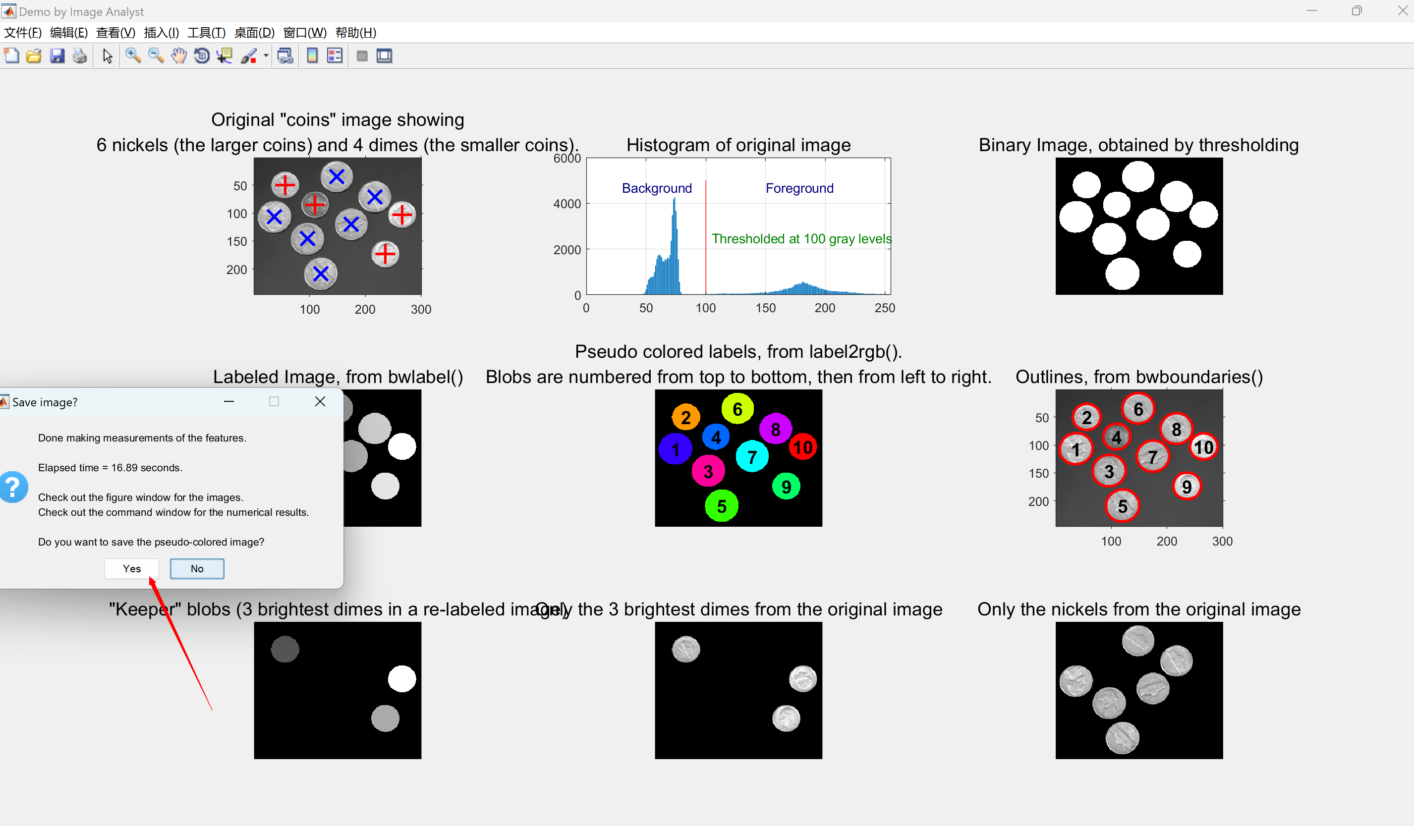
for k = 1 : numberOfBlobs           % Loop through all keeper blobs.% Identify if blob #k is a dime or nickel.itsADime = allBlobAreas(k) < 2200; % Dimes are small.if itsADime% Plot dimes with a red +.plot(centroidsX(k), centroidsY(k), 'r+', 'MarkerSize', 15, 'LineWidth', 2);else% Plot nickels with a blue x.plot(centroidsX(k), centroidsY(k), 'bx', 'MarkerSize', 15, 'LineWidth', 2);end
end%------------------------------------------------------------------------------------------------------------------------------------------------------
% Now use the keeper blobs as a mask on the original image so we will get a masked gray level image.
% This will keep the regions in the mask as original but erase (blacken) everything else (outside of the mask regions).
% This will let us display the original image in the regions of the keeper blobs.
maskedImageDime = originalImage; % Simply a copy at first.
maskedImageDime(~keeperBlobsImage) = 0;	% Set all non-keeper pixels to zero.
subplot(3, 3, 8);
imshow(maskedImageDime);
axis image;
title('Only the 3 brightest dimes from the original image', 'FontSize', captionFontSize);%------------------------------------------------------------------------------------------------------------------------------------------------------
% Now let's get the nickels (the larger coin type).
keeperIndexes = find(allBlobAreas > 2000);  % Take the larger objects.
% Note how we use ismember to select the blobs that meet our criteria.  Get a binary image with only nickel regions present.
nickelBinaryImage = ismember(labeledImage, keeperIndexes);
% Let's get the nickels from the original grayscale image, with the other non-nickel pixels blackened.
% In other words, we will create a "masked" image.
maskedImageNickel = originalImage; % Simply a copy at first.
maskedImageNickel(~nickelBinaryImage) = 0;  % Set all non-nickel pixels to zero.
subplot(3, 3, 9);
imshow(maskedImageNickel, []);
axis image;
title('Only the nickels from the original image', 'FontSize', captionFontSize);%------------------------------------------------------------------------------------------------------------------------------------------------------
% WE'RE BASICALLY DONE WITH THE DEMO NOW.
elapsedTime = toc;
% Alert user that the demo is done and give them the option to save an image.
message = sprintf('Done making measurements of the features.\n\nElapsed time = %.2f seconds.', elapsedTime);
message = sprintf('%s\n\nCheck out the figure window for the images.\nCheck out the command window for the numerical results.', message);
message = sprintf('%s\n\nDo you want to save the pseudo-colored image?', message);
reply = questdlg(message, 'Save image?', 'Yes', 'No', 'No');
% Note: reply will = '' for Upper right X, 'Yes' for Yes, and 'No' for No.
if strcmpi(reply, 'Yes')% Ask user for a filename.FilterSpec = {'*.PNG', 'PNG Images (*.png)'; '*.tif', 'TIFF images (*.tif)'; '*.*', 'All Files (*.*)'};DialogTitle = 'Save image file name';% Get the default filename.  Make sure it's in the folder where this m-file lives.% (If they run this file but the cd is another folder then pwd will show that folder, not this one.thisFile = mfilename('fullpath');[thisFolder, baseFileName, ext] = fileparts(thisFile);DefaultName = sprintf('%s/%s.tif', thisFolder, baseFileName);[fileName, specifiedFolder] = uiputfile(FilterSpec, DialogTitle, DefaultName);if fileName ~= 0% Parse what they actually specified.[folder, baseFileName, ext] = fileparts(fileName);% Create the full filename, making sure it has a tif filename.fullImageFileName = fullfile(specifiedFolder, [baseFileName '.tif']);% Save the labeled image as a tif image.imwrite(uint8(coloredLabels), fullImageFileName);% Just for fun, read image back into the imtool utility to demonstrate that tool.tifimage = imread(fullImageFileName);imtool(tifimage, []);end
end%------------------------------------------------------------------------------------------------------------------------------------------------------
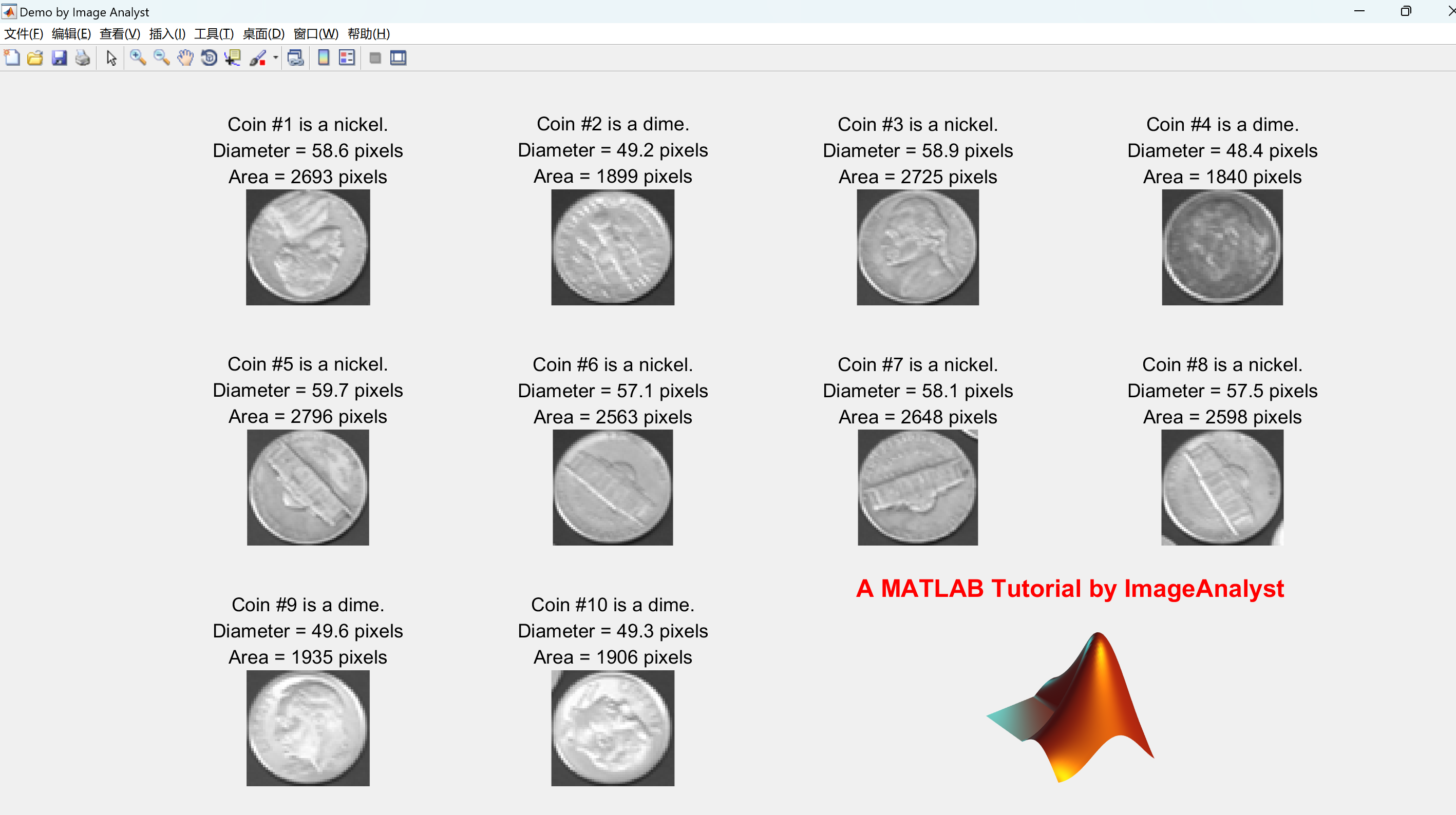
% OPTIONAL : CROP EACH COIN OUT TO A SEPARATE SUB-IMAGE ON A NEW FIGURE.
message = sprintf('Would you like to crop out each coin to individual images?');
reply = questdlg(message, 'Extract Individual Images?', 'Yes', 'No', 'Yes');
% Note: reply will = '' for Upper right X, 'Yes' for Yes, and 'No' for No.
if strcmpi(reply, 'Yes')% Maximize the figure window.hFig2 = figure;	% Create a new figure window.hFig2.Units = 'normalized';hFig2.WindowState = 'maximized'; % Go to full screen.hFig2.NumberTitle = 'off'; % Get rid of "Figure 1"hFig2.Name = 'Demo by Image Analyst'; % Put this into title bar.for k = 1 : numberOfBlobs		% Loop through all blobs.% Find the bounding box of each blob.thisBlobsBoundingBox = props(k).BoundingBox;  % Get list of pixels in current blob.% Extract out this coin into it's own image.subImage = imcrop(originalImage, thisBlobsBoundingBox);% Determine if it's a dime (small) or a nickel (large coin).if props(k).Area > 2200coinType = 'nickel';elsecoinType = 'dime';end% Display the image with informative caption.subplot(3, 4, k);imshow(subImage);caption = sprintf('Coin #%d is a %s.\nDiameter = %.1f pixels\nArea = %d pixels', ...k, coinType, blobECD(k), props(k).Area);title(caption, 'FontSize', textFontSize);end%------------------------------------------------------------------------------------------------------------------------------------------------------% Display the MATLAB "peaks" logo.logoSubplot = subplot(3, 4, 11:12);caption = sprintf('A MATLAB Tutorial by ImageAnalyst');text(0.5,1.15, caption, 'Color','r', 'FontSize', 18, 'FontWeight','b', 'HorizontalAlignment', 'center', 'VerticalAlignment', 'middle') ;positionOfLowerRightPlot = get(logoSubplot, 'position');L = 40*membrane(1,25);logoax = axes('CameraPosition', [-193.4013, -265.1546, 220.4819],...'Box', 'off', ...'CameraTarget',[26, 26, 10], ...'CameraUpVector',[0, 0, 1], ...'CameraViewAngle',9.5, ...'DataAspectRatio', [1, 1, .9],...'Position', positionOfLowerRightPlot, ...'Visible','off', ...'XLim',[1, 51], ...'YLim',[1, 51], ...'ZLim',[-13, 40], ...'parent', gcf);axis(logoSubplot, 'off');s = surface(L, ...'EdgeColor','none', ...'FaceColor',[0.9, 0.2, 0.2], ...'FaceLighting','phong', ...'AmbientStrength',0.3, ...'DiffuseStrength',0.6, ...'Clipping','off',...'BackFaceLighting','lit', ...'SpecularStrength',1, ...'SpecularColorReflectance',1, ...'SpecularExponent',7, ...'Tag','TheMathWorksLogo', ...'parent',logoax);l1 = light('Position',[40, 100, 20], ...

% OPTIONAL : CROP EACH COIN OUT TO A SEPARATE SUB-IMAGE ON A NEW FIGURE.
message = sprintf('Would you like to crop out each coin to individual images?');
reply = questdlg(message, 'Extract Individual Images?', 'Yes', 'No', 'Yes');
% Note: reply will = '' for Upper right X, 'Yes' for Yes, and 'No' for No.
if strcmpi(reply, 'Yes')
   % Maximize the figure window.
   hFig2 = figure;   % Create a new figure window.
   hFig2.Units = 'normalized';
   hFig2.WindowState = 'maximized'; % Go to full screen.
   hFig2.NumberTitle = 'off'; % Get rid of "Figure 1"
   hFig2.Name = 'Demo by Image Analyst'; % Put this into title bar.

   for k = 1 : numberOfBlobs       % Loop through all blobs.
       % Find the bounding box of each blob.
       thisBlobsBoundingBox = props(k).BoundingBox; % Get list of pixels in current blob.
       % Extract out this coin into it's own image.
       subImage = imcrop(originalImage, thisBlobsBoundingBox);
       % Determine if it's a dime (small) or a nickel (large coin).
       if props(k).Area > 2200
           coinType = 'nickel';
       else
           coinType = 'dime';
       end
       % Display the image with informative caption.
       subplot(3, 4, k);
       imshow(subImage);
       caption = sprintf('Coin #%d is a %s.\nDiameter = %.1f pixels\nArea = %d pixels', ...
           k, coinType, blobECD(k), props(k).Area);
       title(caption, 'FontSize', textFontSize);
   end

   %------------------------------------------------------------------------------------------------------------------------------------------------------
   % Display the MATLAB "peaks" logo.
   logoSubplot = subplot(3, 4, 11:12);
   caption = sprintf('A MATLAB Tutorial by ImageAnalyst');
   text(0.5,1.15, caption, 'Color','r', 'FontSize', 18, 'FontWeight','b', 'HorizontalAlignment', 'center', 'VerticalAlignment', 'middle') ;
   positionOfLowerRightPlot = get(logoSubplot, 'position');
   L = 40*membrane(1,25);
   logoax = axes('CameraPosition', [-193.4013, -265.1546, 220.4819],...
       'Box', 'off', ...
       'CameraTarget',[26, 26, 10], ...
       'CameraUpVector',[0, 0, 1], ...
       'CameraViewAngle',9.5, ...
       'DataAspectRatio', [1, 1, .9],...
       'Position', positionOfLowerRightPlot, ...