欢迎来到我的主页:【Echo-Nie】
本篇文章收录于专栏【机器学习】

1 什么是Sigmoid函数?
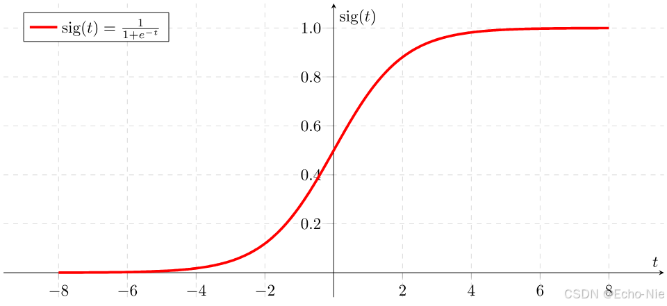
Sigmoid函数(Logistic函数)是机器学习中最经典的激活函数之一,是一个在生物学中常见的S型函数,也称为S型生长曲线。在信息科学中,由于其单增以及反函数单增等性质,常被用作神经网络的激活函数,将变量映射到0,1之间。其数学表达如下:
σ ( x ) = 1 1 + e − x = e x e x + 1 \sigma(x) = \frac{1}{1 + e^{-x}} = \frac{e^x}{e^x + 1} σ(x)=1+e−x1=ex+1ex
函数图像呈现典型的 “S” 形曲线,具有以下特征:
- 定义域: ( − ∞ , + ∞ ) (-\infty, +\infty) (−∞,+∞)
- 值域: ( 0 , 1 ) (0, 1) (0,1)
- 对称性:关于点(0, 0.5)中心对称
- 可导性:处处可导
2 数学性质详解
2.1 导数计算
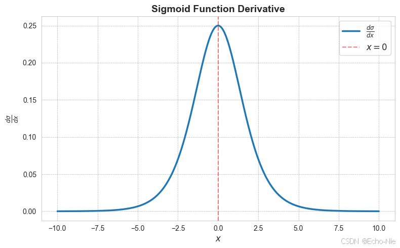
Sigmoid的导数可用其自身表示,这在反向传播中非常关键:
d σ d x = σ ( x ) ( 1 − σ ( x ) ) \frac{d\sigma}{dx} = \sigma(x)(1 - \sigma(x)) dxdσ=σ(x)(1−σ(x))
数学推导:
d d x σ ( x ) = d d x ( 1 1 + e − x ) = e − x ( 1 + e − x ) 2 = 1 1 + e − x ⋅ e − x 1 + e − x = σ ( x ) ( 1 − σ ( x ) ) \begin{aligned} \frac{d}{dx}\sigma(x) &= \frac{d}{dx}\left( \frac{1}{1 + e^{-x}} \right) \\ &= \frac{e^{-x}}{(1 + e^{-x})^2} \\ &= \frac{1}{1 + e^{-x}} \cdot \frac{e^{-x}}{1 + e^{-x}} \\ &= \sigma(x)(1 - \sigma(x)) \end{aligned} dxdσ(x)=dxd(1+e−x1)=(1+e−x)2e−x=1+e−x1⋅1+e−xe−x=σ(x)(1−σ(x))
2.2 重要性质
| 特性 | 说明 |
|---|---|
| 非线性 | 使神经网络可以学习非线性模式 |
| 饱和性 | 当输入绝对值较大时梯度趋近于零 |
| 概率解释 | 输出值可直接解释为概率 |
| 平滑性 | 函数各阶导数均存在,有利于数值计算 |
3 Python实现
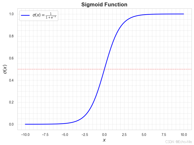
3.1 函数可视化
import numpy as np
import matplotlib.pyplot as plt# 定义Sigmoid函数
def sigmoid(x):return 1 / (1 + np.exp(-x))# 生成x值范围
x = np.linspace(-10, 10, 100)
y = sigmoid(x)plt.figure(figsize=(8, 6))
# 绘制Sigmoid曲线
plt.plot(x, y, label=r'$\sigma(x) = \frac{1}{1 + e^{-x}}$', color='blue', linewidth=2)
plt.title("Sigmoid Function", fontsize=16, fontweight='bold')
plt.xlabel(r"$x$", fontsize=14)
plt.ylabel(r"$\sigma(x)$", fontsize=14)
plt.grid(True, which='both', linestyle='--', linewidth=0.5)
plt.minorticks_on()
plt.tick_params(which='both', width=2)
plt.tick_params(which='major', length=7)
plt.tick_params(which='minor', length=4, color='gray') # 添加水平参考线(y=0.5)
plt.axhline(0.5, color='red', linestyle='--', alpha=0.5, linewidth=1)plt.legend(fontsize=12)
plt.tight_layout()
# 显示图形
plt.show()
3.2 导数可视化
import numpy as np
import matplotlib.pyplot as plt# Sigmoid函数
def sigmoid(x):return 1 / (1 + np.exp(-x))# Sigmoid导数
def sigmoid_derivative(x):s = sigmoid(x)return s * (1 - s)# 生成数据点
x = np.linspace(-10, 10, 400)  # 生成-10到10之间的400个点
dy = sigmoid_derivative(x)     # 计算导数# 绘制Sigmoid导数图
plt.figure(figsize=(8, 5))
plt.plot(x, dy, label=r"$\frac{d\sigma}{dx}$", linewidth=2.5)
plt.title("Sigmoid Function Derivative", fontsize=14, fontweight='bold')
plt.xlabel("$x$", fontsize=12)
plt.ylabel("$\\frac{d\sigma}{dx}$", fontsize=12)
plt.axvline(0, color='red', linestyle='--', alpha=0.5, label="$x=0$")
plt.grid(color='gray', linestyle='--', linewidth=0.5, alpha=0.6)
plt.legend(loc='best', fontsize=12)
plt.tight_layout()
plt.show()
4 应用场景
4.1 逻辑回归做二分类
在逻辑回归中,Sigmoid将线性组合 z = w T x + b z = w^Tx + b z=wTx+b 转换为概率:
P ( y = 1 ∣ x ) = σ ( z ) = 1 1 + e − ( w T x + b ) P(y=1|x) = \sigma(z) = \frac{1}{1 + e^{-(w^Tx + b)}} P(y=1∣x)=σ(z)=1+e−(wTx+b)1
决策边界:当 σ ( z ) ≥ 0.5 \sigma(z) \geq 0.5 σ(z)≥0.5时预测为类别1,等价于 z ≥ 0 z \geq 0 z≥0
from sklearn.linear_model import LogisticRegression
X = [[1.2], [2.4], [3.1], [4.8], [5.0]]
y = [0, 0, 1, 1, 1]
model = LogisticRegression()
model.fit(X, y)
# 预测概率
print(model.predict_proba([[3.0]]))
4.2 神经网络激活函数
虽然现代深度学习更多使用ReLU,但在以下场景仍有用:
- 输出层需要概率输出的分类任务
- LSTM等特殊网络结构的门控机制
- 强化学习的动作选择概率
4.2.1 概率输出的分类任务
在二分类问题中,Sigmoid函数常用于输出层,将线性组合的结果转换为一个介于0到1之间的值,表示样本属于正类的概率。
import torch
import torch.nn as nn
import torch.optim as optim
from sklearn.datasets import make_classification
from sklearn.model_selection import train_test_split
from sklearn.metrics import accuracy_score# 生成二分类数据集
X, y = make_classification(n_samples=1000, n_features=10, n_classes=2, random_state=42)
X_train, X_test, y_train, y_test = train_test_split(X, y, test_size=0.3, random_state=42)# 转换为 PyTorch 张量
X_train = torch.tensor(X_train, dtype=torch.float32)
X_test = torch.tensor(X_test, dtype=torch.float32)
y_train = torch.tensor(y_train, dtype=torch.float32).reshape(-1, 1)
y_test = torch.tensor(y_test, dtype=torch.float32).reshape(-1, 1)# 定义模型
class SimpleNN(nn.Module):def __init__(self):super().__init__()self.fc1 = nn.Linear(10, 5)self.act = nn.Sigmoid()self.fc2 = nn.Linear(5, 1)def forward(self, x):x = self.act(self.fc1(x))return self.fc2(x)# 初始化模型和优化器
model = SimpleNN()
criterion = nn.BCEWithLogitsLoss()  # 二元交叉熵损失
optimizer = optim.Adam(model.parameters(), lr=0.01)# 训练模型
epochs = 100
for epoch in range(epochs):model.train()optimizer.zero_grad()outputs = model(X_train)loss = criterion(outputs, y_train)loss.backward()optimizer.step()if (epoch + 1) % 10 == 0:print(f"Epoch [{epoch + 1}/{epochs}], Loss: {loss.item():.4f}")# 评估模型
model.eval()
with torch.no_grad():y_pred = torch.sigmoid(model(X_test)).round().numpy()
accuracy = accuracy_score(y_test.numpy(), y_pred)
print(f"Test Accuracy: {accuracy:.4f}")
Epoch [10/100], Loss: 0.6665
Epoch [20/100], Loss: 0.6172
Epoch [30/100], Loss: 0.5569
Epoch [40/100], Loss: 0.4926
Epoch [50/100], Loss: 0.4361
Epoch [60/100], Loss: 0.3928
Epoch [70/100], Loss: 0.3627
Epoch [80/100], Loss: 0.3431
Epoch [90/100], Loss: 0.3307
Epoch [100/100], Loss: 0.3229
Test Accuracy: 0.8400
4.2.2 LSTM 网络中的门控机制
import torch
import torch.nn as nnclass SimpleLSTM(nn.Module):def __init__(self, input_size, hidden_size, output_size):super().__init__()self.lstm = nn.LSTM(input_size, hidden_size, batch_first=True)self.fc = nn.Linear(hidden_size, output_size)def forward(self, x):h0 = torch.zeros(1, x.size(0), self.lstm.hidden_size)c0 = torch.zeros(1, x.size(0), self.lstm.hidden_size)out, (hn, cn) = self.lstm(x, (h0, c0))out = self.fc(out[:, -1, :])  # 取最后一个时间步的输出return torch.sigmoid(out)  # 输出概率# 随机数据测试模型
input_size = 10
hidden_size = 5
output_size = 1model = SimpleLSTM(input_size, hidden_size, output_size)
x = torch.randn(32, 5, input_size)  # 32 是 batch_size,5 是序列长度
output = model(x)
print("LSTM output:", output)
LSTM output: tensor([[0.5431],[0.4636],[0.4578],[0.5197],[0.5001],[0.5229],[0.4976],[0.4924],[0.5234],[0.5413],[0.4881],[0.4861],[0.5162],[0.5169],[0.4688],[0.5114],[0.5059],[0.5013],[0.5215],[0.4460],[0.5219],[0.5306],[0.5099],[0.4722],[0.4930],[0.5114],[0.5249],[0.4784],[0.4850],[0.4994],[0.4955],[0.4910]], grad_fn=<SigmoidBackward0>)
4.2.3 强化学习的动作选择概率
举例:预测用户是否会点击某个广告,0 or 1
from sklearn.datasets import make_classification
from sklearn.model_selection import train_test_split
from sklearn.linear_model import LogisticRegression
from sklearn.metrics import accuracy_score, classification_report# 生成模拟数据集
# 特征:用户年龄、浏览历史、广告类型、设备类型
# 标签:是否点击广告(0:未点击,1:点击)
X, y = make_classification(n_samples=1000, n_features=4, n_classes=2, random_state=42)# 划分训练集和测试集
X_train, X_test, y_train, y_test = train_test_split(X, y, test_size=0.3, random_state=42)# 创建逻辑回归模型
model = LogisticRegression()
model.fit(X_train, y_train)# 预测测试集
y_pred = model.predict(X_test)
print("预测结果:", y_pred)# 模型评估
print("准确率:", accuracy_score(y_test, y_pred))
print("分类报告:\n", classification_report(y_test, y_pred))
预测结果: [1 1 0 0 0 1 0 0 0 0 0 1 1 0 1 1 0 0 0 0 1 0 0 1 1 1 1 0 0 1 1 0 1 1 1 1 00 0 1 0 0 0 0 1 0 0 0 0 0 1 0 0 1 1 0 0 0 0 0 0 1 1 0 0 0 1 0 0 1 1 1 1 00 0 1 0 0 1 0 0 1 0 0 0 0 1 1 0 0 1 0 1 1 1 0 1 1 1 0 0 0 1 1 0 0 1 0 0 01 1 0 0 0 1 0 0 1 1 1 1 1 0 1 1 0 1 1 0 1 0 1 0 0 1 1 0 0 0 1 1 1 1 0 1 01 0 0 1 0 0 1 1 0 1 1 0 1 0 1 1 0 0 1 1 1 1 1 0 0 1 1 0 0 0 1 0 1 0 1 0 11 1 0 0 1 0 0 1 0 0 0 1 1 1 1 0 1 1 1 0 0 0 1 1 0 0 1 0 1 0 0 1 0 1 0 0 00 1 1 0 0 1 0 0 1 0 0 0 0 1 0 0 1 0 1 0 1 1 1 0 0 0 0 1 1 1 0 0 0 0 0 1 11 1 0 1 1 0 1 0 0 0 0 0 0 1 1 1 1 0 0 0 0 1 1 0 1 1 0 1 1 1 1 1 0 1 0 0 01 0 1 0]
准确率: 0.8666666666666667
分类报告:precision    recall  f1-score   support0       0.85      0.90      0.87       1531       0.88      0.84      0.86       147accuracy                           0.87       300macro avg       0.87      0.87      0.87       300
weighted avg       0.87      0.87      0.87       300
4.3 数据标准化
将任意范围的特征值压缩到(0,1)区间:
def normalize(values):scaled = (values - np.min(values)) / (np.max(values) - np.min(values))return sigmoid(scaled * 10 - 5)  # 加强非线性缩放original = np.array([10, 20, 30, 40, 50])
print(normalize(original))
5 sklearn代码实战
5.1 基于sklearn的逻辑回归实例
使用 sklearn.datasets 中的 make_classification 数据集,这是一个用于生成二分类或多分类问题的合成数据集。通过该数据集,可以灵活地控制特征数量、类别分布等参数。
数据加载与预处理
from sklearn.datasets import make_classification
from sklearn.model_selection import train_test_split# 生成二分类数据集
X, y = make_classification(n_samples=1000, n_features=2, n_redundant=0, n_clusters_per_class=1, random_state=42)# 划分训练集和测试集,8:2
X_train, X_test, y_train, y_test = train_test_split(X, y, test_size=0.2, random_state=42)
训练模型
from sklearn.linear_model import LogisticRegression
# 逻辑回归模型
model = LogisticRegression()
# 训练模型
model.fit(X_train, y_train)
模型评估
from sklearn.metrics import accuracy_score, confusion_matrix, classification_report
# 预测测试集
y_pred = model.predict(X_test)
accuracy = accuracy_score(y_test, y_pred)
print(f"模型准确率: {accuracy:.2f}")
conf_matrix = confusion_matrix(y_test, y_pred)
print("混淆矩阵:")
print(conf_matrix)
class_report = classification_report(y_test, y_pred)
print("分类报告:")
print(class_report)
模型准确率: 0.90
混淆矩阵:
[[97  7][13 83]]
分类报告:precision    recall  f1-score   support0       0.88      0.93      0.91       1041       0.92      0.86      0.89        96accuracy                           0.90       200
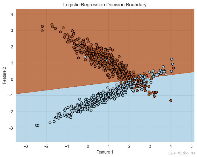
可视化决策边界
import numpy as np
import matplotlib.pyplot as pltx_min, x_max = X[:, 0].min() - 1, X[:, 0].max() + 1
y_min, y_max = X[:, 1].min() - 1, X[:, 1].max() + 1
xx, yy = np.meshgrid(np.arange(x_min, x_max, 0.01),np.arange(y_min, y_max, 0.01))# 预测网格点的类别
Z = model.predict(np.c_[xx.ravel(), yy.ravel()])
Z = Z.reshape(xx.shape)# 绘制决策边界和数据点
plt.figure(figsize=(8, 6))
plt.contourf(xx, yy, Z, alpha=0.8, cmap=plt.cm.Paired)
plt.scatter(X[:, 0], X[:, 1], c=y, edgecolors='k', marker='o', cmap=plt.cm.Paired)
plt.xlabel("Feature 1")
plt.ylabel("Feature 2")
plt.title("Logistic Regression Decision Boundary")
plt.show()
5.2 sklearn乳腺癌数据集
使用 sklearn.datasets 中的 load_breast_cancer 数据集,这是一个用于乳腺癌诊断的二分类数据集。
import numpy as np
import matplotlib.pyplot as plt
from sklearn.datasets import load_breast_cancer
from sklearn.model_selection import train_test_split
from sklearn.linear_model import LogisticRegression
from sklearn.preprocessing import StandardScaler
from sklearn.metrics import roc_curve, auc, accuracy_score, classification_report# 加载乳腺癌数据集
data = load_breast_cancer()
X, y = data.data, data.target# 划分训练集和测试集
X_train, X_test, y_train, y_test = train_test_split(X, y, test_size=0.2, random_state=42)# 数据标准化
scaler = StandardScaler()
X_train_scaled = scaler.fit_transform(X_train)
X_test_scaled = scaler.transform(X_test)# 创建逻辑回归模型
model = LogisticRegression(max_iter=300, solver='lbfgs')
model.fit(X_train_scaled, y_train)# 预测测试集的概率
y_scores = model.predict_proba(X_test_scaled)[:, 1]
y_pred = model.predict(X_test_scaled)print("准确率:", accuracy_score(y_test, y_pred))
print("分类报告:\n", classification_report(y_test, y_pred))# 计算ROC
fpr, tpr, thresholds = roc_curve(y_test, y_scores)
roc_auc = auc(fpr, tpr)# ROC曲线
plt.figure(figsize=(8, 6))
plt.plot(fpr, tpr, color='darkblue', lw=2, label=f'ROC curve (AUC = {roc_auc:.2f})')
plt.plot([0, 1], [0, 1], color='gray', lw=2, linestyle='--')
plt.xlim([0.0, 1.0])
plt.ylim([0.0, 1.05])
plt.xlabel('False Positive Rate', fontsize=14)
plt.ylabel('True Positive Rate', fontsize=14)
plt.title('Receiver Operating Characteristic (ROC) Curve', fontsize=16)
plt.legend(loc='lower right', fontsize=12)
plt.grid(color='lightgray', linestyle='--', linewidth=0.5)
plt.gca().spines['top'].set_color('none')
plt.gca().spines['right'].set_color('none')
plt.gca().spines['bottom'].set_linewidth(1.2)
plt.gca().spines['left'].set_linewidth(1.2)
plt.gca().tick_params(axis='both', which='major', labelsize=12)
plt.tight_layout()
plt.show()
准确率: 0.9736842105263158
分类报告:precision    recall  f1-score   support0       0.98      0.95      0.96        431       0.97      0.99      0.98        71accuracy                           0.97       114macro avg       0.97      0.97      0.97       114
weighted avg       0.97      0.97      0.97       114