M-estimators
在这里我们研究一种叫M-estimators的渐进高斯性。具体来说,如果参数估计可以用一个最小化或者最大化目标表示:
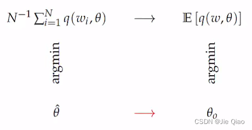
θ o = arg min θ ∈ Θ E [ q ( w , θ ) ] \theta _{o} =\arg\min_{\theta \in \Theta }\mathbb{E}[ q(w,\theta )] θo=argθ∈ΘminE[q(w,θ)]
比如最大似然估计就是最大化似然函数的参数,那么把样本代进去,我们就可以得到m-estimator(maximum-likelihood-like estimator Huber (1967)):
θ ^ = arg min θ N − 1 ∑ i = 1 N q ( w i , θ ) \hat{\theta } =\arg\min_{\theta } N^{-1}\sum _{i=1}^{N} q(w_{i} ,\theta ) θ^=argθminN−1i=1∑Nq(wi,θ)
它表示就是从样本中估计的参数。
我们也可以用其极值条件来表示这个估计量,即找到其导数为0的极值点就是我们的 θ ^ \displaystyle \hat{\theta } θ^:
N − 1 ∑ i = 1 N ∇ θ q ( w i , θ ^ ) = 0 N^{-1}\sum _{i=1}^{N} \nabla _{\theta } q(w_{i} ,\hat{\theta } )=0 N−1i=1∑N∇θq(wi,θ^)=0
这个估计方式也被称为generalized method of moments(GMM),大部分情况下GMM和MLE是等价的,GMM的适用范围会更广一点,因为那些无法用MLE的模型可以用GMM来求,比如有些数据的分布不知道,或者写不出具体的形式,这时候MLE就没法用了。
Consistency and normality of M-estimators
那么这个估计的参数 θ ^ \displaystyle \hat{\theta } θ^有些什么性质呢?对于估计量的性质,我们一般关心这三个问题:可识别性(identifiability),一致性(consistency),以及渐进高斯性(asymptotic normality)。
可识别性是基本要求,也就是这个极值点是唯一的,不可以存在另外的参数但他们的大小相同,这个性质一般是具体问题具体分析,这里先假设成立。
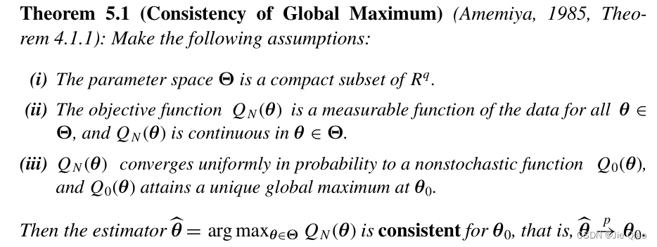
Consistency
对于一致性,其实就是 θ ^ → p θ 0 \displaystyle \hat{\theta }\xrightarrow{p} \theta _{0} θ^pθ0是否依概率收敛到到真实的 θ 0 \displaystyle \theta _{0} θ0上去。
为了证明一致性,如上图,我们可以以他们的目标函数作为桥梁,通过证明 N − 1 ∑ i = 1 N q ( w i , θ ) \displaystyle N^{-1}\sum _{i=1}^{N} q(w_{i} ,\theta ) N−1i=1∑Nq(wi,θ)uniform convergence收敛到 E [ q ( w , θ ) ] \displaystyle E[ q( w,\theta )] E[q(w,θ)](其实就是大数定理),并且基于 θ 0 \displaystyle \theta _{0} θ0的可识别性,以及连续有界等等性质,证明出 θ ^ → p θ 0 \displaystyle \hat{\theta }\xrightarrow{p} \theta _{0} θ^pθ0:
Normality
最后是渐进高斯性,所谓渐进高斯就是
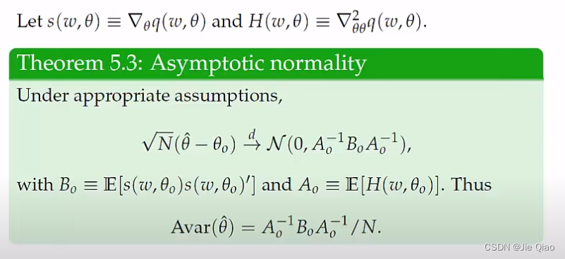
这个定理告诉我们,这个估计的参数是服从正态分布的,而且他的方差取决于q的一阶和二阶导数。这东西是怎么来的呢,其实就是通过泰勒展开建立了估计参数与目标函数导数的桥梁。具体推导如下,这里都假设可识别性以及一致性成立。
首先定义符号, s i ( θ ) \displaystyle s_{i} (\theta ) si(θ)是一个 1 × P 1\times P 1×P 向量
s i ( θ ) ≡ ∇ θ q ( w i , θ ) = ( ∂ q ( w i , θ ) ∂ θ 1 , . . . , ∂ q ( w i , θ ) ∂ θ P ) T \begin{array}{ r c l } s_{i} (\theta ) & \equiv & \nabla _{\theta } q(w_{i} ,\theta )\\ & = & \left(\frac{\partial q(w_{i} ,\theta )}{\partial \theta _{1}} ,...,\frac{\partial q(w_{i} ,\theta )}{\partial \theta _{P}}\right)^{T} \end{array} si(θ)≡=∇θq(wi,θ)(∂θ1∂q(wi,θ),...,∂θP∂q(wi,θ))T
H i ( θ ) \displaystyle H_{i} (\theta ) Hi(θ)则是 P × P P\times P P×P矩阵
H i ( θ ) ≡ ∇ θ θ 2 q ( w i , θ ) = ∂ 2 q ( w i , θ ) ∂ θ ∂ θ ′ . H_{i} (\theta )\equiv \nabla _{\theta \theta }^{2} q(w_{i} ,\theta )=\frac{\partial ^{2} q(w_{i} ,\theta )}{\partial \theta \partial \theta ^{\prime }} . Hi(θ)≡∇θθ2q(wi,θ)=∂θ∂θ′∂2q(wi,θ).
接下来我们希望对 s i ( θ ) \displaystyle s_{i}( \theta ) si(θ)作一阶泰勒展开。回顾一下泰勒展开,一个连续函数 f ( x ) \displaystyle f( x) f(x)在 x 0 \displaystyle x_{0} x0处的展开为:
f ( x ) = f ( x 0 ) + f ′ ( x + ) ( x − x 0 ) f(x)=f(x_{0} )+f'(x^{+} )(x-x_{0} ) f(x)=f(x0)+f′(x+)(x−x0)
其中 x + \displaystyle \ x^{+} x+是 x 0 \displaystyle x_{0} x0和 x \displaystyle x x之间的数,这个也称为中值定理。但如果f的输出是个向量,那么这个展开就是向量形式的泰勒展开:
f ( x ) = f ( x 0 ) + ∂ f ( x ) ∂ x ∣ x = x + ( x − x 0 ) \mathbf{f} (\mathbf{x} )=\mathbf{f} (\mathbf{x}_{0} )+\frac{\partial \mathbf{f} (\mathbf{x} )}{\partial \mathbf{x}}\Bigl|_{\mathbf{x} =\mathbf{x}^{+}} (\mathbf{x} -\mathbf{x}_{0} ) f(x)=f(x0)+∂x∂f(x) x=x+(x−x0)
这里 ∂ f ( x ) ∂ x \displaystyle \frac{\partial \mathbf{f} (\mathbf{x} )}{\partial \mathbf{x}} ∂x∂f(x)是一个矩阵,对于该矩阵的每一行,其对应的 x + \displaystyle \mathbf{x}^{+} x+都是不同的。
接下来,我们建立 θ \displaystyle \theta θ与 s ( θ ) \displaystyle s( \theta ) s(θ)的联系,具体的,把这个泰勒展开用到 s i ( θ ) \displaystyle s_{i} (\theta ) si(θ)上,
∑ i = 1 N s i ( θ ^ ) = ∑ i = 1 N s i ( θ 0 ) + ∑ i = 1 N ∂ s i ( θ ) ∂ θ ∣ θ + ( θ ^ − θ 0 ) \sum _{i=1}^{N} s_{i} (\hat{\theta } )=\sum _{i=1}^{N} s_{i} (\theta _{0} )+\sum _{i=1}^{N}\frac{\partial s_{i} (\theta )}{\partial \theta }\Bigl|_{\theta ^{+}} (\hat{\theta } -\theta _{0} ) i=1∑Nsi(θ^)=i=1∑Nsi(θ0)+i=1∑N∂θ∂si(θ) θ+(θ^−θ0)
现在,我们用 S ( θ ) = 1 N ∑ i = 1 N s i ( θ ) = 1 N ∑ i = 1 N ∇ θ q ( w i , θ ) \displaystyle S( \theta ) =\frac{1}{N}\sum _{i=1}^{N} s_{i} (\theta )=\frac{1}{N}\sum _{i=1}^{N} \nabla _{\theta } q(w_{i} ,\theta ) S(θ)=N1i=1∑Nsi(θ)=N1i=1∑N∇θq(wi,θ), S ′ ( θ ) = 1 N ∑ i = 1 N ∂ s i ( θ ) ∂ θ ∣ θ + = 1 N ∑ i = 1 N ∇ θ θ 2 q ( w i , θ ) \displaystyle S'( \theta ) =\frac{1}{N}\sum _{i=1}^{N}\frac{\partial s_{i} (\theta )}{\partial \theta }\Bigl|_{\theta ^{+}} =\frac{1}{N}\sum _{i=1}^{N} \nabla _{\theta \theta }^{2} q(w_{i} ,\theta ) S′(θ)=N1i=1∑N∂θ∂si(θ) θ+=N1i=1∑N∇θθ2q(wi,θ),于是
S ( θ ^ ) = S ( θ 0 ) + S ′ ( θ + ) ( θ ^ − θ 0 ) S(\hat{\theta }) =S( \theta _{0}) +S'\left( \theta ^{+}\right) (\hat{\theta } -\theta _{0} ) S(θ^)=S(θ0)+S′(θ+)(θ^−θ0)
首先,根据 θ ^ \displaystyle \hat{\theta } θ^的定义,他是通过极值点求得的,因此 S ( θ ^ ) = 0 \displaystyle S(\hat{\theta }) =0 S(θ^)=0,于是
0 = S ( θ 0 ) + S ′ ( θ + ) ( θ ^ − θ 0 ) θ ^ − θ 0 = − S ′ ( θ + ) − 1 S ( θ 0 ) \begin{aligned} 0 & =S( \theta _{0}) +S'\left( \theta ^{+}\right) (\hat{\theta } -\theta _{0} )\\ \hat{\theta } -\theta _{0} & =-S'\left( \theta ^{+}\right)^{-1} S( \theta _{0}) \end{aligned} 0θ^−θ0=S(θ0)+S′(θ+)(θ^−θ0)=−S′(θ+)−1S(θ0)
接下来,希望将 θ + \displaystyle \theta ^{+} θ+变成 θ 0 \displaystyle \theta _{0} θ0。基于参数的一致性 θ ^ → p θ 0 \displaystyle \hat{\theta }\xrightarrow{p} \theta _{0} θ^pθ0,并且进一步假设 S ′ \displaystyle S' S′这个函数是平滑的,那么就会有
θ ^ − θ 0 = − S ′ ( θ 0 ) − 1 S ( θ 0 ) + o p ( 1 ) N ( θ ^ − θ 0 ) = − S ′ ( θ 0 ) − 1 N S ( θ 0 ) ⏟ → N ( 0 , B 0 ) + o p ( 1 ) \begin{aligned} \hat{\theta } -\theta _{0} & =-S'( \theta _{0})^{-1} S( \theta _{0}) +o_{p}( 1)\\ \sqrt{N}(\hat{\theta } -\theta _{0}) & =-S'( \theta _{0})^{-1}\underbrace{\sqrt{N} S( \theta _{0})}_{\rightarrow \mathcal{N}( 0,B_{0})} +o_{p}( 1) \end{aligned} θ^−θ0N(θ^−θ0)=−S′(θ0)−1S(θ0)+op(1)=−S′(θ0)−1→N(0,B0) NS(θ0)+op(1)
这里 o p ( 1 ) \displaystyle o_{p}( 1) op(1)表示这条等式在 N → ∞ \displaystyle N\rightarrow \infty N→∞的时候成立。接下来,因为 θ 0 \displaystyle \theta _{0} θ0是个常数,而 S ( θ 0 ) = 1 N ∑ i = 1 N ∇ θ q ( w i , θ 0 ) \displaystyle S( \theta _{0}) =\frac{1}{N}\sum _{i=1}^{N} \nabla _{\theta } q(w_{i} ,\theta _{0} ) S(θ0)=N1i=1∑N∇θq(wi,θ0),是一个样本的均值,所以根据中心极限定理,这个东西会趋于正态分布,并且因为 E [ S ( θ 0 ) ] = 0 \displaystyle E[ S( \theta _{0})] =0 E[S(θ0)]=0(因为 θ 0 \displaystyle \theta _{0} θ0是 E [ q ( w , θ ) ] \displaystyle \mathbb{E}[ q(w,\theta )] E[q(w,θ)]的极值点),所以其正态分布的均值为0,而其方差则是 V a r ( ∇ θ q ( w i , θ 0 ) ) = V a r ( s i ( θ 0 ) ) \displaystyle Var( \nabla _{\theta } q(w_{i} ,\theta _{0} )) =Var( s_{i} (\theta _{0} )) Var(∇θq(wi,θ0))=Var(si(θ0)),记为 B 0 \displaystyle B_{0} B0,并且记 A 0 : = S ′ ( θ 0 ) \displaystyle A_{0} :=S'( \theta _{0}) A0:=S′(θ0)
N ( θ ^ − θ 0 ) → d N ( 0 , A 0 − 1 B 0 A 0 − 1 ) \sqrt{N}(\hat{\theta } -\theta _{0})\xrightarrow{d}\mathcal{N}\left( 0,A_{0}^{-1} B_{0} A_{0}^{-1}\right) N(θ^−θ0)dN(0,A0−1B0A0−1)
这里之所以两个 A 0 \displaystyle A_{0} A0是因为 − a ∗ N ( 0 , 1 ) ∼ N ( 0 , a 2 ) \displaystyle -a*N( 0,1) \sim N\left( 0,a^{2}\right) −a∗N(0,1)∼N(0,a2),是矩阵的平方的写法。最后这就是我们的定理
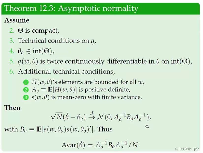
我们发现,这个参数估计的方差是取决于 V a r ( ∇ θ q ( w i , θ 0 ) ) \displaystyle Var( \nabla _{\theta } q(w_{i} ,\theta _{0} )) Var(∇θq(wi,θ0))以及 E [ ∇ θ θ 2 q ( w i , θ ) ] \displaystyle E\left[ \nabla _{\theta \theta }^{2} q(w_{i} ,\theta )\right] E[∇θθ2q(wi,θ)].
这个证明核心的地方是那个泰勒展开,其导数 S ( θ 0 ) \displaystyle S( \theta _{0}) S(θ0)是样本均值求和,根据中心极限定理是渐进高斯的,又因为参数 θ ^ − θ 0 \displaystyle \hat{\theta } -\theta _{0} θ^−θ0可以用 S ( θ 0 ) \displaystyle S( \theta _{0}) S(θ0)表示,从而可以写出渐进高斯的表达式。
例子
考虑一个简单的线性模型
y = a x + ϵ , y=ax+\epsilon ,\ y=ax+ϵ,
其中 x ∼ N ( 0 , σ x 2 ) , ϵ ∼ N ( 0 , σ ϵ 2 ) \displaystyle x\sim \mathcal{N}\left( 0,\sigma _{x}^{2}\right) ,\epsilon \sim \mathcal{N}\left( 0,\sigma _{\epsilon }^{2}\right) x∼N(0,σx2),ϵ∼N(0,σϵ2)。于是,
a ^ = arg max 1 N ∑ i = 1 N log p ( x i , y i ; a ) = arg min 1 N ∑ i = 1 N ( y i − a x i ) 2 \begin{aligned} \hat{a} & =\arg\max\frac{1}{N}\sum _{i=1}^{N}\log p( x_{i} ,y_{i} ;a)\\ & =\arg\min\frac{1}{N}\sum _{i=1}^{N}( y_{i} -ax_{i})^{2} \end{aligned} a^=argmaxN1i=1∑Nlogp(xi,yi;a)=argminN1i=1∑N(yi−axi)2
因此, q ( x i , y i , a ) = ( y i − a x i ) 2 \displaystyle q( x_{i} ,y_{i} ,a) =( y_{i} -ax_{i})^{2} q(xi,yi,a)=(yi−axi)2,于是
B 0 = V a r ( ∇ a q ( x i , y i , a ) ) = V a r ( − 2 ( y i − a x i ) x i ) = V a r ( − 2 ϵ i x i ) = E [ 4 ϵ i 2 x i 2 ] − 4 E [ ϵ i x i ] 2 = 4 σ x 2 σ ϵ 2 A 0 = E [ ∇ a a 2 q ( x i , y i , a ) ] = E [ 2 x i 2 ] = 2 σ x 2 B_{0} =Var( \nabla _{a} q( x_{i} ,y_{i} ,a)) =Var( -2( y_{i} -ax_{i}) x_{i}) =Var( -2\epsilon _{i} x_{i}) =E\left[ 4\epsilon _{i}^{2} x_{i}^{2}\right] -4E[ \epsilon _{i} x_{i}]^{2} =4\sigma _{x}^{2} \sigma _{\epsilon }^{2}\\ A_{0} =E\left[ \nabla _{aa}^{2} q( x_{i} ,y_{i} ,a)\right] =E\left[ 2x_{i}^{2}\right] =2\sigma _{x}^{2} B0=Var(∇aq(xi,yi,a))=Var(−2(yi−axi)xi)=Var(−2ϵixi)=E[4ϵi2xi2]−4E[ϵixi]2=4σx2σϵ2A0=E[∇aa2q(xi,yi,a)]=E[2xi2]=2σx2
于是,我们有
N ( a ^ − a ) → d N ( 0 , σ ϵ 2 σ x 2 ) \sqrt{N}(\hat{a} -a)\xrightarrow{d}\mathcal{N}\left( 0,\frac{\sigma _{\epsilon }^{2}}{\sigma _{x}^{2}}\right) N(a^−a)dN(0,σx2σϵ2)
参考资料
Consistency and normality of M-estimators
Linearity of the Integrator of Riemann-Stieltjes Integrals