channel $h_k$ is modeled as independent Rayleigh fading with average power loss set as 10^−3

Python

import numpy as np# Set the parameters
average_power_loss = 1e-3  # Average power loss (10^(-3))
num_samples = 1000  # Number of fading samples to generate# Calculate the Rayleigh scale parameter (sigma)
# The scale parameter is related to the average power loss as follows:
# average_power_loss = 2 * sigma^2
sigma = np.sqrt(average_power_loss / 2)# Generate independent Rayleigh fading samples
rayleigh_samples = sigma * np.random.randn(num_samples) + 1j * sigma * np.random.randn(num_samples)# The above code generates complex samples, where the real and imaginary parts
# are both independently Rayleigh distributed.# Optionally, you can plot a histogram of the fading samples to visualize
# the Rayleigh distribution.
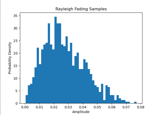
import matplotlib.pyplot as pltplt.hist(np.abs(rayleigh_samples), bins=50, density=True)
plt.title("Rayleigh Fading Samples")
plt.xlabel("Amplitude")
plt.ylabel("Probability Density")
plt.show()

对比一下：

H = np.random.rayleigh(scale=1, size= N)*1e-3

如果设定的hk是实数，直接取模就行了。

# Take the absolute value to get real Rayleigh fading samples
rayleigh_samples_real = np.abs(rayleigh_samples_complex)

Matlab:

% Set the average power loss
average_power_loss = 10^(-3);% Calculate the scale parameter (σ)
sigma = sqrt(average_power_loss / 2);% Number of samples to generate
num_samples = 1000;% Generate random samples from the Rayleigh distribution
rayleigh_samples = raylrnd(sigma, 1, num_samples);% Plot the histogram of the generated samples
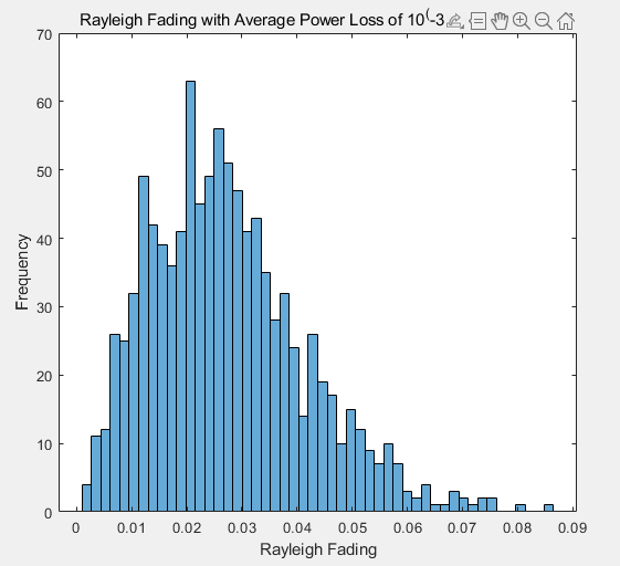
histogram(rayleigh_samples, 50); % Adjust the number of bins as needed% Label the axes
xlabel('Rayleigh Fading');
ylabel('Frequency');% Title for the plot
title(['Rayleigh Fading with Average Power Loss of 10^(-3), \sigma = ', num2str(sigma)]);