【机器学习】几种常用的机器学习调参方法

在机器学习中，模型的性能往往受到模型的超参数、数据的质量、特征选择等因素影响。其中，模型的超参数调整是模型优化中最重要的环节之一。超参数（Hyperparameters）在机器学习算法中需要人为设定，它们不能直接从训练数据中学习得出。与之对应的是模型参数（Model Parameters），它们是模型内部学习得来的参数。
以支持向量机（SVM）为例，其中C、kernel 和 gamma 就是超参数，而通过数据学习到的权重 w 和偏置 b则是模型参数。实际应用中，我们往往需要选择合适的超参数才能得到一个好的模型。搜索超参数的方法有很多种，如网格搜索、随机搜索、对半网格搜索、贝叶斯优化、遗传算法、模拟退火等方法，具体内容如下。

一、网格搜索

网格搜索可能是最简单、应用最广泛的超参数搜索算法，通过查找搜索范围内的所有的点来确定最优值。如果采用较大的搜索范围以及较小的步长，网恪搜索很大概率找到全局最优值。然而，这种搜索方案十分消耗计算资源和时间，特别是需要调优的超参数比较多的时候。
因此，在实际应用中，网格搜索法一般会先使用较广的搜索范围和较大的步长，来寻找全局最优值可能的位置。然后通过逐渐缩小搜索范围和步长，来寻找更精确的最优值。这种操作方案可以降低所需的时间和计算量，但由于目标函数一般是非凸的，所以很可能会错过全局最优值。

import time
from sklearn.model_selection import KFold
from sklearn.ensemble import RandomForestClassifierrf_param_grid = {'max_depth' : list(range(2,20,2)),'n_estimators': list(range(20,800,100)),'min_samples_split': [2,6,10],'min_samples_leaf': [2,6,10]}

#计算参数空间大小
def count_space(rf_param_grid):no_option=1for i in rf_param_grid:no_option*=len(rf_param_grid[i])return no_option
count_space(rf_param_grid)

参数空间总量为648个。

#网格搜索GridSearchCV
from sklearn.model_selection import GridSearchCV
start_time = time.time() 
m = RandomForestClassifier(n_jobs = -1, random_state = 2023)
cv = KFold(n_splits = 5, shuffle = True, random_state = 2023)
m_g = GridSearchCV(param_grid=rf_param_grid,estimator = m,scoring = "roc_auc",cv = cv)
m_g.fit(x_train, y_train)
end_time = time.time() 
run_time = end_time - start_time
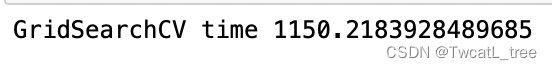
print("GridSearchCV time", run_time)

在这里插入图片描述

for key in m_r.best_params_.keys():print('%s = %s'%(key,m_g.best_params_[key]))

在这里插入图片描述


y_pred_train = m_g.predict_proba(x_train)[:,1]
fpr_train,tpr_train,_ = roc_curve(y_train,y_pred_train)
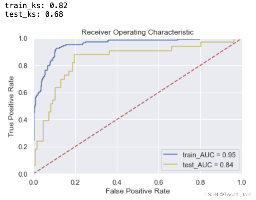
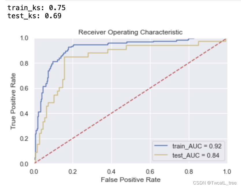
train_ks = round(abs(fpr_train-tpr_train).max(), 2)
roc_auc_train = auc(fpr_train, tpr_train)
print('train_ks:',train_ks)y_pred = m_g.predict_proba(x_test)[:,1]
fpr_test, tpr_test,_ = roc_curve(y_test,y_pred)
test_ks = round(abs(fpr_test-tpr_test).max(), 2)
roc_auc_test = auc(fpr_test, tpr_test)
print('test_ks:',test_ks)plt.title('Receiver Operating Characteristic')
plt.plot(fpr_train, tpr_train, 'b', label = 'train_AUC = %0.2f' % roc_auc_train)
plt.plot(fpr_test, tpr_test, 'y', label = 'test_AUC = %0.2f' % roc_auc_test)
plt.legend(loc = 'lower right')
plt.plot([0, 1], [0, 1],'r--')
plt.xlim([0, 1])
plt.ylim([0, 1])
plt.ylabel('True Positive Rate')
plt.xlabel('False Positive Rate')
plt.show()

在这里插入图片描述

二、随机搜索

随机搜索的思想与网格搜索比较相似，只是不再测试上界和下界之间的所有值，而是在搜索范围中随机选取样本点。它的理论依据是，如果样本点集足够大，那么通过随机采样也能大概率地找到全局最优值，或其近似值。随机搜索一般会比网格搜索要快一些，但是和网格搜索的快速版一样，它的结果也是没法保证的。

# 随机搜索RandomizedSearchCV
from sklearn.model_selection import RandomizedSearchCV
m = RandomForestClassifier(n_jobs = -1, random_state = 2023)
cv = KFold(n_splits = 5, shuffle = True, random_state = 2023)m_r = RandomizedSearchCV(param_distributions=rf_param_grid,estimator = m,scoring = "roc_auc",cv = cv,n_iter=10,verbose=True,n_jobs=-1)
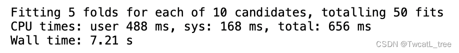
%time  m_r.fit(x_train, y_train)

在这里插入图片描述


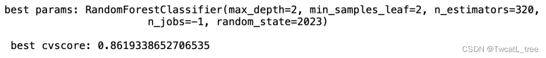
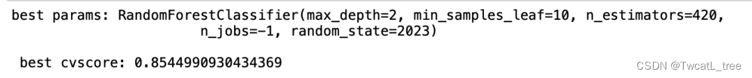
print("best params:", m_r.best_estimator_, "\n","\n", "best cvscore:", m_r.best_score_)

在这里插入图片描述


y_pred_train = m_r.predict_proba(x_train)[:,1]
fpr_train,tpr_train,_ = roc_curve(y_train,y_pred_train)
train_ks = round(abs(fpr_train-tpr_train).max(), 2)
roc_auc_train = auc(fpr_train, tpr_train)
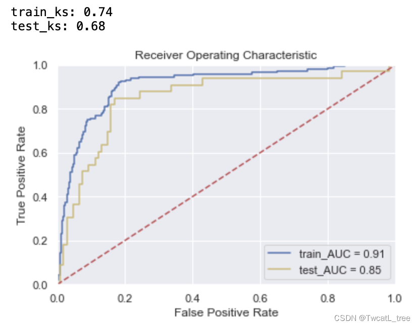
print('train_ks:',train_ks)y_pred = m_r.predict_proba(x_test)[:,1]
fpr_test, tpr_test,_ = roc_curve(y_test,y_pred)
test_ks = round(abs(fpr_test-tpr_test).max(), 2)
roc_auc_test = auc(fpr_test, tpr_test)
print('test_ks:',test_ks)plt.title('Receiver Operating Characteristic')
plt.plot(fpr_train, tpr_train, 'b', label = 'train_AUC = %0.2f' % roc_auc_train)
plt.plot(fpr_test, tpr_test, 'y', label = 'test_AUC = %0.2f' % roc_auc_test)
plt.legend(loc = 'lower right')
plt.plot([0, 1], [0, 1],'r--')
plt.xlim([0, 1])
plt.ylim([0, 1])
plt.ylabel('True Positive Rate')
plt.xlabel('False Positive Rate')
plt.show()

在这里插入图片描述

三、对半网格搜索

面对枚举网格搜索过慢的问题，sklearn中呈现了两种优化方式：其一是调整搜索空间，其二是调整每次训练的数据。调整搜索空间的方法就是随机网格搜索，而调整每次训练数据的方法就是对半网格搜索。
假设现在有数据集D，我们从数据集D中随机抽样出一个子集d。如果一组参数在整个数据集D上表现较差，那大概率这组参数在数据集的子集d上表现也不会太好。反之，如果一组参数在子集d上表现不好，我们也不会信任这组参数在全数据集D上的表现。那么我们可以认为参数在子集与在全数据集上的表现一致。
但在现实数据中，这一假设要成立是有条件的，即任意子集的分布都与全数据集D的分布类似。当子集的分布越接近全数据集的分布，同一组参数在子集与全数据集上的表现越有可能一致。根据之前在随机网格搜索中得出的结论，我们知道子集越大、其分布越接近全数据集的分布，但是大子集又会导致更长的训练时间，因此为了整体训练效率，我们不可能无限地增大子集。这就出现了一个矛盾：大子集上的结果更可靠，但大子集计算更缓慢。
对半网格搜索算法设计了一个精妙的流程，可以很好的权衡子集的大小与计算效率问题，具体流程如下：
首先从全数据集中无放回随机抽样出一个很小的子集 d0 ，并在d0上验证全部参数组合的性能。根据d0上的验证结果，淘汰评分排在后1/2的那一半参数组合。然后，从全数据集中再无放回抽样出一个比 d0大一倍的子集 d1，并在d1上验证剩下的那一半参数组合的性能。根据 d1上的验证结果，淘汰评分排在后1/2的参数组合。再从全数据集中无放回抽样出一个比 d1大一倍的子集 d2，并在 d2上验证剩下1/4的参数组合的性能。根据 d2上的验证结果，淘汰评分排在后1/2的参数组合……，直至到达限制条件。
在这种模式下，只有在不同的子集上不断获得优秀结果的参数组合能够被留存到迭代的后期，最终选择出的参数组合一定是在所有子集上都表现优秀的参数组合。这样一个参数组合在全数据上表现优异的可能性是非常大的，同时也可能展现出比网格、随机搜索得出的参数更大的泛化能力。
然而这个过程当中会存在一个问题：子集越大时，子集与全数据集D的分布会越相似，但整个对半搜索算法在开头的时候，就用最小的子集筛掉了最多的参数组合。如果最初的子集与全数据集的分布差异很大，那么在对半搜索开头的前几次迭代中，就可能筛掉许多对全数据集D有效的参数，因此对半网格搜索最初的子集一定不能太小。

# 对半网格搜索HalvingGridSearchCV
from sklearn.experimental import enable_halving_search_cv
from sklearn.model_selection import HalvingGridSearchCVm = RandomForestClassifier(n_jobs = -1, random_state = 2023)
cv = KFold(n_splits = 5, shuffle = True, random_state = 2023)
m_h = HalvingGridSearchCV(estimator = m,param_grid=rf_param_grid,factor=3,min_resources = 100,scoring='roc_auc',n_jobs = -1,random_state=2023,cv=cv)
%time m_h.fit(x_train, y_train)

print("best params:", m_h.best_estimator_, "\n","\n", "best cvscore:", m_h.best_score_)

y_pred_train = m_h.predict_proba(x_train)[:,1]
fpr_train,tpr_train,_ = roc_curve(y_train,y_pred_train)
train_ks = round(abs(fpr_train-tpr_train).max(), 2)
roc_auc_train = auc(fpr_train, tpr_train)
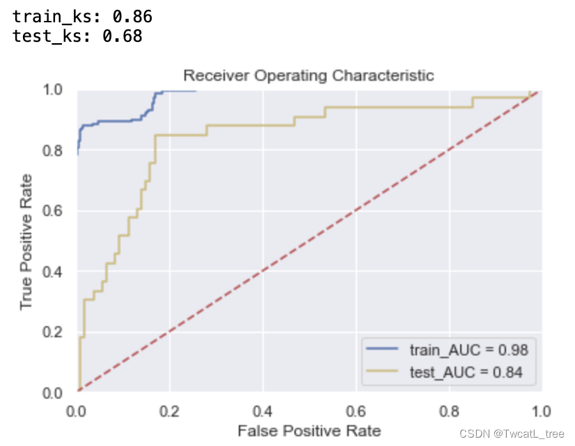
print('train_ks:',train_ks)y_pred = m_h.predict_proba(x_test)[:,1]
fpr_test, tpr_test,_ = roc_curve(y_test,y_pred)
test_ks = round(abs(fpr_test-tpr_test).max(), 2)
roc_auc_test = auc(fpr_test, tpr_test)
print('test_ks:',test_ks)plt.title('Receiver Operating Characteristic')
plt.plot(fpr_train, tpr_train, 'b', label = 'train_AUC = %0.2f' % roc_auc_train)
plt.plot(fpr_test, tpr_test, 'y', label = 'test_AUC = %0.2f' % roc_auc_test)
plt.legend(loc = 'lower right')
plt.plot([0, 1], [0, 1],'r--')
plt.xlim([0, 1])
plt.ylim([0, 1])
plt.ylabel('True Positive Rate')
plt.xlabel('False Positive Rate')
plt.show()

四、贝叶斯优化

贝叶斯优化算法在寻找最优值参数时，采用了与网格搜索、随机搜索完全不同的方法。网格搜索和随机搜索在测试一个新点时，会忽略前一个点的信息，而贝叶斯优化算法则充分利用了之前的信息。贝叶斯优化算法通过对目标函数形状进行学习，找到使目标函数向全局最优值提升的参数。
具体来说，它学习目标函数形状的方法是，首先根据先验分布，假设一个搜集函数，每一次使用新的采样点来测试目标函数时，利用这个信息来更新目标函数的先验分布；最后，算法测试由后验分布给出的全局最值最可能出现的位置的点。
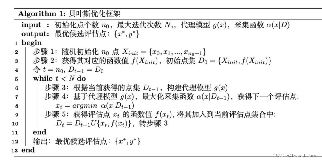
对于贝叶斯优化算法，有一个需要注意的地方，一旦找到了一个局部最优值，它会在该区域不断采样，所以很容易陷入局部最优值。为了弥补这个缺陷，贝叶斯优化算法会在探索和利用之间找到一个平衡点，“探索”就是在还未取样的区域获取采样点；而“利用”则是根据后验分布在最可能出现全局最值的区域进行采样。下图为贝叶斯优化框架：

4.1基于高斯过程的贝叶斯优化

bayes-optimization是最早开源的贝叶斯优化库之一，也是为数不多至今依然保留着高斯过程优化的优化库。

#贝叶斯优化Baysian optimization
##BayesianOptimization只支持目标函数最大值，不支持最小值
from bayes_opt import BayesianOptimizationdef randomforest_evaluate(**params):params['max_depth'] = int(round(params['max_depth'],0))params['n_estimators'] = int(round(params['n_estimators'],0))params['min_samples_split'] = int(round(params['min_samples_split'],0))params['min_samples_leaf'] = int(round(params['min_samples_leaf'],0))model = RandomForestClassifier(**params, n_jobs=-1, random_state = 2023)cv = KFold(n_splits = 5, shuffle = True, random_state = 2023)validation_loss = cross_validate(model, x_train, y_train,scoring='roc_auc',cv = cv,verbose=False,n_jobs=-1,error_score='raise')       return np.mean(validation_loss['test_score'])

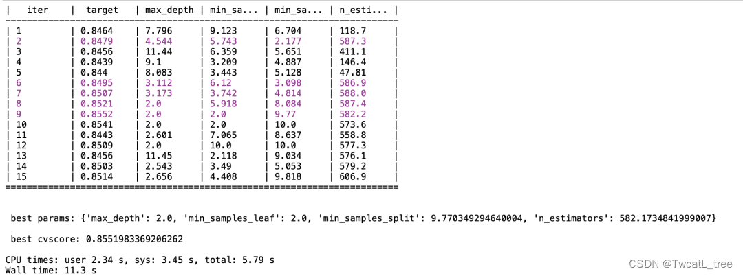
rf_param_grid = {'max_depth' : (2,20),'n_estimators': (20,800),'min_samples_split': (2,10),'min_samples_leaf': (2, 10)}def param_bayes_opt(init_points, n_iter):opt = BayesianOptimization(randomforest_evaluate, rf_param_grid, random_state=2023)opt.maximize(init_points = init_points, n_iter = n_iter)params_best = opt.max['params']score_best = opt.max['target']print("\n","\n", "best params:", params_best,"\n","\n", "best cvscore:", score_best,"\n")%time param_bayes_opt(5, 10)

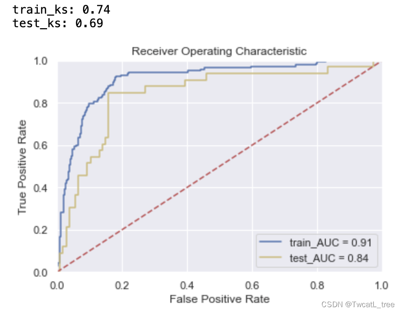
m_o = RandomForestClassifier(max_depth = 2,min_samples_leaf = 2,min_samples_split = 9,n_estimators = 582,n_jobs = -1,random_state = 2023).fit(x_train, y_train)y_pred_train = m_o.predict_proba(x_train)[:,1]
fpr_train,tpr_train,_ = roc_curve(y_train,y_pred_train)
train_ks = round(abs(fpr_train-tpr_train).max(), 2)
roc_auc_train = auc(fpr_train, tpr_train)
print('train_ks:',train_ks)y_pred = m_o.predict_proba(x_test)[:,1]
fpr_test, tpr_test,_ = roc_curve(y_test,y_pred)
test_ks = round(abs(fpr_test-tpr_test).max(), 2)
roc_auc_test = auc(fpr_test, tpr_test)
print('test_ks:',test_ks)plt.title('Receiver Operating Characteristic')
plt.plot(fpr_train, tpr_train, 'b', label = 'train_AUC = %0.2f' % roc_auc_train)
plt.plot(fpr_test, tpr_test, 'y', label = 'test_AUC = %0.2f' % roc_auc_test)
plt.legend(loc = 'lower right')
plt.plot([0, 1], [0, 1],'r--')
plt.xlim([0, 1])
plt.ylim([0, 1])
plt.ylabel('True Positive Rate')
plt.xlabel('False Positive Rate')
plt.show()

4.2基于TPE的贝叶斯优化
Hyperopt优化器是目前最为通用的贝叶斯优化器之一，Hyperopt中集成了包括随机搜索、模拟退火和TPE（Tree-structured Parzen Estimator Approach）等多种优化算法。可通过参数algo指定搜索算法，如随机搜索hyperopt.rand.suggest、模拟退火hyperopt.anneal.suggest、TPE算法hyperopt.tpe.suggest。

相比于Bayes_opt，Hyperopt的是更先进、更现代、维护更好的优化器，也是我们最常用来实现TPE方法的优化器。在实际使用中，相比基于高斯过程的贝叶斯优化，基于高斯混合模型的TPE在大多数情况下以更高效率获得更优结果，该方法目前也被广泛应用于AutoML领域中。

#贝叶斯优化Tree of Parzen Estimators (TPE) 
#Hyperopt只支持寻找目标函数的最小值，不支持寻找最大值
from hyperopt import hp, fmin, tpe, Trials, partial
from hyperopt.early_stop import no_progress_loss# 设定参数空间
space = {'max_depth': hp.quniform('max_depth', 2,20, 2),'n_estimators': hp.quniform('n_estimators', 20, 800, 50),'min_samples_split' : hp.choice('min_samples_split',[2,3,6,9,10]),'min_samples_leaf' : hp.choice('min_samples_leaf',[2,3,6,9,10])}# 设定目标函数_基评估器选择随机森林
def randomforest_evaluate(params):model = RandomForestClassifier(n_estimators = int(params["n_estimators"]),max_depth = int(params["max_depth"]),min_samples_split = int(params["min_samples_split"]),min_samples_leaf = params["min_samples_leaf"],n_jobs=-1, random_state = 2023)cv = KFold(n_splits = 5, shuffle = True, random_state = 2023)validation_loss = cross_validate(model, x_train, y_train,scoring='roc_auc',cv = cv,verbose = False,n_jobs = -1,error_score = 'raise')       return np.mean((-1) * validation_loss['test_score'])def param_hyperopt(max_evals):#记录迭代过程trials=Trials()#提前停止early_stop_fn=no_progress_loss(100) #定义代理模型params_best=fmin(randomforest_evaluate,space=space ,algo=tpe.suggest,max_evals=max_evals,trials=trials ,early_stop_fn=early_stop_fn)if params_best["min_samples_split"] <=1:params_best["min_samples_split"] = 2if params_best["min_samples_split"] <=1:params_best["min_samples_leaf"] = 2print('best parmas:',params_best)return params_best,trials%time params_best, trials=param_hyperopt(30)

m_t = RandomForestClassifier(max_depth = 2,min_samples_leaf = 4,min_samples_split = 4,n_estimators = 350,n_jobs = -1,random_state = 2023).fit(x_train, y_train)y_pred_train = m_t.predict_proba(x_train)[:,1]
fpr_train,tpr_train,_ = roc_curve(y_train,y_pred_train)
train_ks = round(abs(fpr_train-tpr_train).max(), 2)
roc_auc_train = auc(fpr_train, tpr_train)
print('train_ks:',train_ks)y_pred = m_t.predict_proba(x_test)[:,1]
fpr_test, tpr_test,_ = roc_curve(y_test,y_pred)
test_ks = round(abs(fpr_test-tpr_test).max(), 2)
roc_auc_test = auc(fpr_test, tpr_test)
print('test_ks:',test_ks)plt.title('Receiver Operating Characteristic')
plt.plot(fpr_train, tpr_train, 'b', label = 'train_AUC = %0.2f' % roc_auc_train)
plt.plot(fpr_test, tpr_test, 'y', label = 'test_AUC = %0.2f' % roc_auc_test)
plt.legend(loc = 'lower right')
plt.plot([0, 1], [0, 1],'r--')
plt.xlim([0, 1])
plt.ylim([0, 1])
plt.ylabel('True Positive Rate')
plt.xlabel('False Positive Rate')
plt.show()

五、遗传算法
受生物进化论的启发，1975年J.Holland提出遗传算法（Genetic Algorithm，GA）。GA是一种基于“适者生存”的高度并行、随机和自适应优化的搜索算法，它将问题的求解表示成“染色体”的适者生存过程。通过“染色体”群的一代代不断进化，使用复制（reproduction）、交叉（crossover）和变异（mutation）等操作，最终收敛到“最适应环境”的个体，从而求得问题最优解。
本文遗传算法调参使用Tree-based Pipeline Optimization Tool库（TPOT，基于树的管道优化工具）。TPOT 基于树的结构来表示预测建模问题的模型管道，包括数据准备和建模算法以及模型超参数。它利用流行的 Scikit-Learn 机器学习库进行数据转换和机器学习算法，并使用遗传编程随机全局搜索过程来有效地发现给定数据集的性能最佳的模型管道。

from tpot import TPOTClassifiern_estimators = [10,11,12,13,14,15,16]
max_depth = [5,10,20,30,40,50,60]
criterion=['entropy', 'gini']
min_samples_leaf=[1, 2, 5, 10]
min_samples_split=[2, 5, 10, 15]
max_features = ['auto', 'sqrt','log2']param = {'n_estimators': n_estimators,'max_features': max_features,'max_depth': max_depth,'min_samples_split': min_samples_split,'min_samples_leaf': min_samples_leaf,'criterion':['entropy','gini']}tpot_classifier = TPOTClassifier(generations= 5, population_size= 24, offspring_size= 12,verbosity= 2, early_stop= 12,config_dict={'sklearn.ensemble.RandomForestClassifier': param}, cv = 4, scoring = 'roc_auc')
%time tpot_classifier.fit(x_train,y_train)

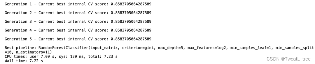
m_a = RandomForestClassifier(max_depth = 5,min_samples_leaf = 1,min_samples_split = 10,n_estimators = 11,criterion='gini',n_jobs = -1,random_state = 2023).fit(x_train, y_train)y_pred_train = m_a.predict_proba(x_train)[:,1]
fpr_train,tpr_train,_ = roc_curve(y_train,y_pred_train)
train_ks = round(abs(fpr_train-tpr_train).max(), 2)
roc_auc_train = auc(fpr_train, tpr_train)
print('train_ks:',train_ks)y_pred = m_a.predict_proba(x_test)[:,1]
fpr_test, tpr_test,_ = roc_curve(y_test,y_pred)
test_ks = round(abs(fpr_test-tpr_test).max(), 2)
roc_auc_test = auc(fpr_test, tpr_test)
print('test_ks:',test_ks)plt.title('Receiver Operating Characteristic')
plt.plot(fpr_train, tpr_train, 'b', label = 'train_AUC = %0.2f' % roc_auc_train)
plt.plot(fpr_test, tpr_test, 'y', label = 'test_AUC = %0.2f' % roc_auc_test)
plt.legend(loc = 'lower right')
plt.plot([0, 1], [0, 1],'r--')
plt.xlim([0, 1])
plt.ylim([0, 1])
plt.ylabel('True Positive Rate')
plt.xlabel('False Positive Rate')
plt.show()