本文仅供学习使用
本文参考:
B站:CLEAR_LAB
笔者带更新-运动学
课程主讲教师:
Prof. Wei Zhang
课程链接 :
https://www.wzhanglab.site/teaching/mee-5114-advanced-control-for-robotics/
南科大高等机器人控制课 Ch12 Robotic Motion Control
- 1. Basic Linear Control Design
- 1.1 Error Response
- 1.2 Standard Second-Order Systems
- 1.3 Second-Order Response Characteristics
- 1.4 State-Space Controller Design
- 2. Motion Control Problems
- 2.1 Robotic Motion Control Problem
- 2.2 Variations in Robot Motion Control
- 3. Motion Control with Velocity/Acceleration as Input
- 3.1 Velocity-Resolved Control
- 3.2.1 Velocity-Resolved Joint Space Control
- 3.2.2 Velocity-Resolved Task Space Control
- 3.2 Acceleration-Resolved Control
- 3.2.1 Acceleration-Resolved Control in Joint Space
- 3.2.2 Acceleration-Resolved Control in Task Space
- 4. Motion Control with Torque as Input and Task Space Inverse Dynamics
- 4.1 Recall Properties of Robot Dynamics
- 4.2 Computed Torque Control
- 4.3 Inverse Dynamics Control
机器人——运动能力、计算能力、感知决策能力 的机电系统
1. Basic Linear Control Design
1.1 Error Response

Steady-state error : e s s = lim t → ∞ θ e ( t ) e_{\mathrm{ss}}=\underset{t\rightarrow \infty}{\lim}\theta _{\mathrm{e}}\left( t \right) ess=t→∞limθe(t)
Precent overshoot : P.O.
Rise time / Peak time :
Settling time : T s T_{\mathrm{s}} Ts
1.2 Standard Second-Order Systems
详细推导见 : (待补充)

1.3 Second-Order Response Characteristics
详细推导见 : (待补充)

1.4 State-Space Controller Design

- Eigenvalue assignment : Find control gain K K K such that e i g ( A − B K ) = e i g d e s i r e d eig\left( A-BK \right) =eig_{\mathrm{desired}} eig(A−BK)=eigdesired
- Solvability : We can always find such K K K if ( A , B ) \left( A,B \right) (A,B) is controllable ( r a n k ( m c ) = n rank\left( m_{\mathrm{c}} \right) =n rank(mc)=n)
- How to choose desired eigs? —— refer to 2nd-order system
specification (P.O. T s T_{\mathrm{s}} Ts T p T_{\mathrm{p}} Tp) ⇒ a r t \overset{art}{\Rightarrow} ⇒art dominant poles + other poles ⇒ \Rightarrow ⇒ e i g d e s i r e d eig_{\mathrm{desired}} eigdesired ⇒ s c i e n c e \overset{science}{\Rightarrow} ⇒science K K K
2. Motion Control Problems
2.1 Robotic Motion Control Problem
Dynamic equation of fully-acuated robot (with external force) : { τ = M ( q ) q ¨ + c ( q , q ˙ ) q ˙ + g ( q ) + J T ( q ) F e x t y = h ( q ) \begin{cases} \tau =M\left( q \right) \ddot{q}+c\left( q,\dot{q} \right) \dot{q}+g\left( q \right) +J^{\mathrm{T}}\left( q \right) \mathcal{F} _{\mathrm{ext}}\\ y=h\left( q \right)\\ \end{cases} {τ=M(q)q¨+c(q,q˙)q˙+g(q)+JT(q)Fexty=h(q)
q ∈ R n q\in \mathbb{R} ^n q∈Rn : joint positions (generalized coordinate)
τ ∈ R n \tau \in \mathbb{R} ^n τ∈Rn : joint torque (generalized input)
y y y : output (variable to be controlled) —— can be any func of q q q , e.g. y = q , y = [ T ( q ) ] ∈ S E ( 3 ) y=q,y=\left[ T\left( q \right) \right] \in SE\left( 3 \right) y=q,y=[T(q)]∈SE(3)
- Motion Control Problems : Let y y y track given reference y d y_{\mathrm{d}} yd
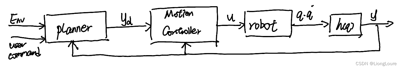
often times q d q_{\mathrm{d}} qd is given by planner represented by polynomials , so that q ˙ d , q ¨ d \dot{q}_{\mathrm{d}},\ddot{q}_{\mathrm{d}} q˙d,q¨d can be easily obtained
2.2 Variations in Robot Motion Control
-
Joint-space vs. Task-space control
Joint-space : y ( t ) = q ( t ) y\left( t \right) =q\left( t \right) y(t)=q(t) , i.e. , want q ( t ) q\left( t \right) q(t) to track a given q d ( t ) q_{\mathrm{d}}\left( t \right) qd(t) joint reference
Task-space : y ( t ) = [ T ( q ( t ) ) ] ∈ S E ( 3 ) y\left( t \right) =\left[ T\left( q\left( t \right) \right) \right] \in SE\left( 3 \right) y(t)=[T(q(t))]∈SE(3) denotes end-effector pose/configuration, we want y ( t ) y\left( t \right) y(t) to track y d ( t ) y_{\mathrm{d}}\left( t \right) yd(t) -
Actuation models:
Velocity source : u = q ˙ u=\dot{q} u=q˙ —— directly control velocity
Acceleration sources : u = q ¨ u=\ddot{q} u=q¨ —— directly control acceleration
Torque sources : u = τ u=\tau u=τ —— directly control torque

Acutation model make sense if for ant given u u u , the joint velocity q ˙ \dot{q} q˙ can immediatly reach u u u
Motion Control Problem
Design u u u to set y y y track desired reference y d y_{\mathrm{d}} yd
- Depending on our assumption on u / y u/y u/y
output y y y —— 6大基本问题
y ↔ q ∈ R n y\leftrightarrow q\in \mathbb{R} ^n y↔q∈Rn - joint variable : Joint space motion control (Velocity-resolved Joint-space control ; Acceleration-resolved Joint-space control ; Torque-resolved Joint-space control ; )
y ↔ [ T ( q ) ] ∈ S E ( 3 ) y\leftrightarrow \left[ T\left( q \right) \right] \in SE\left( 3 \right) y↔[T(q)]∈SE(3) or y = f ( q ) y=f\left( q \right) y=f(q) - task space variable - e.g. origin of end-effector frame : Task space motion control (Velocity-resolved Task-space ; Acceleration-resolved Task-space ; Torque-resolved Task-space ; )
Linear control / feedback lineariazation
3. Motion Control with Velocity/Acceleration as Input
3.1 Velocity-Resolved Control
Each joints’ velocity q ˙ i \dot{q}_{\mathrm{i}} q˙i can be directly controlled
Good approximation for hydraulic actuators
Common approxiamtion of the outer-loop control for the Inner / outer loop control setup

3.2.1 Velocity-Resolved Joint Space Control
Joint-space ‘dynamics’ : single integrator q ˙ = u \dot{q}=u q˙=u
Joint-space tracking becomes standard linear tracking control problem : u = q ˙ d + K 0 q ¨ ⇒ q ~ ˙ + K 0 q ¨ = 0 u=\dot{q}_{\mathrm{d}}+K_0\ddot{q}\Rightarrow \dot{\tilde{q}}+K_0\ddot{q}=0 u=q˙d+K0q¨⇒q~˙+K0q¨=0 , where q ~ = q d − q \tilde{q}=q_{\mathrm{d}}-q q~=qd−q is the joint position error. —— stable if e i g ( − K 0 ) ∈ O L H P eig\left( -K_0 \right) \in OLHP eig(−K0)∈OLHP
The error dynamic is stable if − K 0 -K_0 −K0 is Hurwitz
3.2.2 Velocity-Resolved Task Space Control
For task space control , y = [ T ( q ) ] y=\left[ T\left( q \right) \right] y=[T(q)] needs to track y d y_{\mathrm{d}} yd , y y y can be ant function of q q q, in particular , it can represents position and/or the end-effector frame
Taking derivatives of y y y , and letting u = q ˙ u=\dot{q} u=q˙ , we have : y ˙ = J a ( q ) u \dot{y}=J_{\mathrm{a}}\left( q \right) u y˙=Ja(q)u
Note that q q q is function of y y y through inverse kinematics ( q = I K ( y ) q=IK\left( y \right) q=IK(y))
So the above dynamics can be written in terms of y y y and u u u only. The detailed form can be quite complex in general y ˙ = J a ( I K ( y ) ) u \dot{y}=J_{\mathrm{a}}\left( IK\left( y \right) \right) u y˙=Ja(IK(y))u
- Let v y v_{\mathrm{y}} vy be virtual control y ˙ = v y \dot{y}=v_{\mathrm{y}} y˙=vy design v y v_{\mathrm{y}} vy to track y d y_{\mathrm{d}} yd (same as above)
- Find actual control u u u such that J a ( I K ( y ) ) u ≈ v y J_{\mathrm{a}}\left( IK\left( y \right) \right) u\approx v_{\mathrm{y}} Ja(IK(y))u≈vy


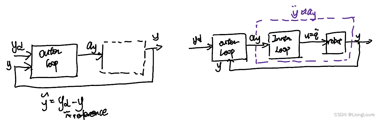
We can design outer-loop controller as if we can directly control y ˙ \dot{y} y˙
y ˙ = v y = y ˙ d + K ( y d − y ) ⟹ p l u g i n y ˙ = v y y ~ ˙ = − K y ~ \dot{y}=v_{\mathrm{y}}=\dot{y}_{\mathrm{d}}+K\left( y_{\mathrm{d}}-y \right) \overset{plug\,\,in\,\,\dot{y}=v_{\mathrm{y}}\,\,}{\Longrightarrow}\dot{\tilde{y}}=-K\tilde{y} y˙=vy=y˙d+K(yd−y)⟹pluginy˙=vyy~˙=−Ky~
We can select K K K such that − K -K −K is Hurtwiz , object of inner loop : determine u = q ˙ u=\dot{q} u=q˙ such that y ˙ ≈ v y \dot{y}\approx v_{\mathrm{y}} y˙≈vy
System(2) is nonlinear system , a commeon way is to break it into inner-outer loop , where the outer loop directly control velocity of y y y, and the inner loop tries to find u u u to generate desired task space velocity
Outer loop : y ˙ = v y \dot{y}=v_{\mathrm{y}} y˙=vy , where control v y = y ˙ d + K 0 y ~ v_{\mathrm{y}}=\dot{y}_{\mathrm{d}}+K_0\tilde{y} vy=y˙d+K0y~ , resulting in task-space closed-loop error dynamics: y ~ ˙ + K 0 y ~ = 0 \dot{\tilde{y}}+K_0\tilde{y}=0 y~˙+K0y~=0
Above task space tracking relies on a fictitious control v y v_{\mathrm{y}} vy , i.e. , it assumes y ˙ \dot{y} y˙ can be arbitrarily controlled by selecting appropriate u = q ˙ u=\dot{q} u=q˙ , which is true if J a J_{\mathrm{a}} Ja is full-row rank
Inner loop : Given v y v_{\mathrm{y}} vy from the outer loop, find the joint velocity control by solving
{ min u ∥ v y − J a ( q ) u ∥ 2 + r e g u l a r i z a t i o n t e r m s u b j . t o : C o n s t r a i n t s o n u , e . g . { q ˙ min ⩽ u ⩽ q ˙ max q min ⩽ q + u Δ t ⩽ q max \begin{cases} \min _{\mathrm{u}}\left\| v_{\mathrm{y}}-J_{\mathrm{a}}\left( q \right) u \right\| ^2+regularization\,\,term\\ subj.to\,\,: Constraints\,\,on\,\,u\,\,, e.g.\begin{cases} \dot{q}_{\min}\leqslant u\leqslant \dot{q}_{\max}\\ q_{\min}\leqslant q+u\varDelta t\leqslant q_{\max}\\ \end{cases}\\ \end{cases} ⎩ ⎨ ⎧minu∥vy−Ja(q)u∥2+regularizationtermsubj.to:Constraintsonu,e.g.{q˙min⩽u⩽q˙maxqmin⩽q+uΔt⩽qmax
Inner-loop is essentially a differential IK controller
One can also use the pseudo-inverse control u = J a † v y u={J_{\mathrm{a}}}^{\dagger}v_{\mathrm{y}} u=Ja†vy
3.2 Acceleration-Resolved Control
3.2.1 Acceleration-Resolved Control in Joint Space
Joint acceleration cna be directly controlled , resulting in double-integrator dynamics q ¨ = u \ddot{q}=u q¨=u . Given q d q_{\mathrm{d}} qd reference , we want q → q d q\rightarrow q_{\mathrm{d}} q→qd (double integartor)
Joint-space tracking becomes standard linear tracking control problem for double-integrator system:
u = q ¨ d + K 1 q ~ ˙ + K 0 q ~ = 0 , q ~ ∈ R n u=\ddot{q}_{\mathrm{d}}+K_1\dot{\tilde{q}}+K_0\tilde{q}=0,\tilde{q}\in \mathbb{R} ^n u=q¨d+K1q~˙+K0q~=0,q~∈Rn
—— PD control , closed-loop system , where q ~ = q d − q \tilde{q}=q_{\mathrm{d}}-q q~=qd−q is the joint position error.
Stablility condition : Let x = [ q ~ q ~ ˙ ] ∈ R 2 n x=\left[ \begin{array}{c} \tilde{q}\\ \dot{\tilde{q}}\\ \end{array} \right] \in \mathbb{R} ^{2n} x=[q~q~˙]∈R2n , [ 0 E − K 0 − K 1 ] [ q ~ q ~ ˙ ] , x ˙ = A x \left[ \begin{matrix} 0& E\\ -K_0& -K_1\\ \end{matrix} \right] \left[ \begin{array}{c} \tilde{q}\\ \dot{\tilde{q}}\\ \end{array} \right] ,\dot{x}=Ax [0−K0E−K1][q~q~˙],x˙=Ax
closed-loop system is stable . if e i g ( A ) ∈ O L H P eig\left( A \right) \in OLHP eig(A)∈OLHP or A A A is Hurwitz
3.2.2 Acceleration-Resolved Control in Task Space
For task space control , y = [ T ( q ) ] ∈ S E ( 3 ) y=\left[ T\left( q \right) \right] \in SE\left( 3 \right) y=[T(q)]∈SE(3) needs to track y d y_{\mathrm{d}} yd

Note : For y = f ( q ) y=f\left( q \right) y=f(q) y ˙ = J a ( q ) q ˙ \dot{y}=J_{\mathrm{a}}\left( q \right) \dot{q} y˙=Ja(q)q˙ and y ¨ = J ˙ a ( q ) q ˙ + J a ( q ) q ¨ ⇒ y ¨ = J ˙ a ( q ) q ˙ + J a ( q ) u ⇐ \ddot{y}=\dot{J}_{\mathrm{a}}\left( q \right) \dot{q}+J_{\mathrm{a}}\left( q \right) \ddot{q}\Rightarrow \ddot{y}=\dot{J}_{\mathrm{a}}\left( q \right) \dot{q}+J_{\mathrm{a}}\left( q \right) u\Leftarrow y¨=J˙a(q)q˙+Ja(q)q¨⇒y¨=J˙a(q)q˙+Ja(q)u⇐ nonlinear dynamics
Following the same inner-outer loop strategy deiscussed before . Introduce virtual control , a y a_{\mathrm{y}} ay such that y ¨ = a y \ddot{y}=a_{\mathrm{y}} y¨=ay , we can design controller for a y a_{\mathrm{y}} ay to let y → y d y\rightarrow y_{\mathrm{d}} y→yd
Outer-loop dynamics : y ¨ = a y \ddot{y}=a_{\mathrm{y}} y¨=ay , with a y a_{\mathrm{y}} ay being the outer-loop control input a y = y ¨ d + K 1 y ~ ˙ + K 0 y ~ ⇒ y ~ ¨ + K 1 y ~ ˙ + K 0 y ~ = 0 a_{\mathrm{y}}=\ddot{y}_{\mathrm{d}}+K_1\dot{\tilde{y}}+K_0\tilde{y}\Rightarrow \ddot{\tilde{y}}+K_1\dot{\tilde{y}}+K_0\tilde{y}=0 ay=y¨d+K1y~˙+K0y~⇒y~¨+K1y~˙+K0y~=0
—— PD control , stable if [ 0 E − K 0 − K 1 ] \left[ \begin{matrix} 0& E\\ -K_0& -K_1\\ \end{matrix} \right] [0−K0E−K1] Hurwitz
Inner-loop : given a y a_{\mathrm{y}} ay from outer loop , find the “best” joint acceleration:
{ min u ∥ a y − J ˙ a ( q ) q ˙ − J a ( q ) u ∥ 2 + r e g u l a r i z a t i o n t e r m s u b j . t o : C o n s t r a i n t s o n u \begin{cases} \min _{\mathrm{u}}\left\| a_{\mathrm{y}}-\dot{J}_{\mathrm{a}}\left( q \right) \dot{q}-J_{\mathrm{a}}\left( q \right) u \right\| ^2+regularization\,\,term\\ subj.to\,\,: Constraints\,\,on\,\,u\,\,\\ \end{cases} ⎩ ⎨ ⎧minu ay−J˙a(q)q˙−Ja(q)u 2+regularizationtermsubj.to:Constraintsonu
—— u u u : optimization variable , J ˙ a ( q ) , q ˙ , q \dot{J}_{\mathrm{a}}\left( q \right) ,\dot{q},q J˙a(q),q˙,q - known
{ A c c : q ¨ min ⩽ u ⩽ q ¨ max V e l : q ˙ min ⩽ q + u Δ t ⩽ q ˙ max \begin{cases} Acc\,\,: \ddot{q}_{\min}\leqslant u\leqslant \ddot{q}_{\max}\\ Vel\,\,: \dot{q}_{\min}\leqslant q+u\varDelta t\leqslant \dot{q}_{\max}\\ \end{cases} {Acc:q¨min⩽u⩽q¨maxVel:q˙min⩽q+uΔt⩽q˙max
Mathematically , the above problem is the same as the Differential IK problem
At any given time , q ˙ , q \dot{q},q q˙,q can be measured , and then y , y ˙ y,\dot{y} y,y˙ can be computed, which allows us to compute outer loop control a y a_{\mathrm{y}} ay and inner loop control u u u
4. Motion Control with Torque as Input and Task Space Inverse Dynamics
4.1 Recall Properties of Robot Dynamics
For fully actuated robot :
τ = M ( q ) q ¨ + C ( q , q ˙ ) q ˙ + g ( q ) \tau =M\left( q \right) \ddot{q}+C\left( q,\dot{q} \right) \dot{q}+g\left( q \right) τ=M(q)q¨+C(q,q˙)q˙+g(q)
M ( q ) = ∑ J i T [ I i ] 6 × 6 J i ∈ R n × n M\left( q \right) =\sum{{J_{\mathrm{i}}}^{\mathrm{T}}\left[ \mathcal{I} _{\mathrm{i}} \right] _{6\times 6}J_{\mathrm{i}}}\in \mathbb{R} ^{n\times n} M(q)=∑JiT[Ii]6×6Ji∈Rn×n
There are many valid difinitions of C ( q , q ˙ ) C\left( q,\dot{q} \right) C(q,q˙) , typical choice for C C C include:
C i j = ∑ k 1 2 ( ∂ M i j ∂ q k + ∂ M i k ∂ q j − ∂ M j k ∂ q i ) C_{\mathrm{ij}}=\sum_k^{}{\frac{1}{2}\left( \frac{\partial M_{\mathrm{ij}}}{\partial q_{\mathrm{k}}}+\frac{\partial M_{\mathrm{ik}}}{\partial q_{\mathrm{j}}}-\frac{\partial M_{\mathrm{jk}}}{\partial q_{\mathrm{i}}} \right)} Cij=∑k21(∂qk∂Mij+∂qj∂Mik−∂qi∂Mjk)
For the above defined C C C , we have M ˙ − 2 C \dot{M}-2C M˙−2C is skew symmetric
For all valid C C C, we have q ˙ T [ M ˙ − 2 C ] q ˙ = 0 \dot{q}^{\mathrm{T}}\left[ \dot{M}-2C \right] \dot{q}=0 q˙T[M˙−2C]q˙=0
These properties play improtant role in designing motion controller
4.2 Computed Torque Control
For fully-actuated robot, we have M ( q ) ≻ 0 M\left( q \right) \succ 0 M(q)≻0 and q ¨ \ddot{q} q¨ can be arbitrarily specified through torque control u = τ u=\tau u=τ
q ¨ = M − 1 ( q ) [ u − C ( q , q ˙ ) q ˙ − g ( q ) ] \ddot{q}=M^{-1}\left( q \right) \left[ u-C\left( q,\dot{q} \right) \dot{q}-g\left( q \right) \right] q¨=M−1(q)[u−C(q,q˙)q˙−g(q)]
we know how to design controller if u = q ¨ u=\ddot{q} u=q¨

Thus , for fully-acuated robot, torque controlled case can be reduced to the acceleration-resolved case
Outer loop: q ¨ = a q \ddot{q}=a_{\mathrm{q}} q¨=aq with joint acceleration as control input
a q = q ¨ + K 1 y ~ ˙ + K 0 y ~ ⇒ q ~ ¨ + K 1 q ~ ˙ + K 0 q ~ = 0 a_{\mathrm{q}}=\ddot{q}+K_1\dot{\tilde{y}}+K_0\tilde{y}\Rightarrow \ddot{\tilde{q}}+K_1\dot{\tilde{q}}+K_0\tilde{q}=0 aq=q¨+K1y~˙+K0y~⇒q~¨+K1q~˙+K0q~=0
Inner loop : since M ( q ) M\left( q \right) M(q) is square and nonsingular , inner loop control u u u can be found analytically:
u = M ( q ) ( q ¨ d + K 1 q ~ ˙ + K 0 q ~ ) + C ( q , q ˙ ) q ˙ + g ( q ) u=M\left( q \right) \left( \ddot{q}_{\mathrm{d}}+K_1\dot{\tilde{q}}+K_0\tilde{q} \right) +C\left( q,\dot{q} \right) \dot{q}+g\left( q \right) u=M(q)(q¨d+K1q~˙+K0q~)+C(q,q˙)q˙+g(q)

The control law is a function of q , q ˙ q,\dot{q} q,q˙ and the reference q d q_{\mathrm{d}} qd. It is called computed-torque control.
The control law also relies on system model M , C , g M,C,g M,C,g if these model information are not accurate, the control will not perform well.
y = f ( q ) , y ¨ = J ˙ a ( q ) q ˙ + J a ( q ) M − 1 ( u − C − g ) y=f\left( q \right) ,\ddot{y}=\dot{J}_{\mathrm{a}}\left( q \right) \dot{q}+J_{\mathrm{a}}\left( q \right) M^{-1}\left( u-C-g \right) y=f(q),y¨=J˙a(q)q˙+Ja(q)M−1(u−C−g)
Idea easily extends to task space : y ˙ = J a ( q ) q ˙ \dot{y}=J_{\mathrm{a}}\left( q \right) \dot{q} y˙=Ja(q)q˙ and y ¨ = J ˙ a ( q ) q ˙ + J a ( q ) q ¨ \ddot{y}=\dot{J}_{\mathrm{a}}\left( q \right) \dot{q}+J_{\mathrm{a}}\left( q \right) \ddot{q} y¨=J˙a(q)q˙+Ja(q)q¨ —— τ = u = τ , q ¨ = M − 1 [ u − C − g ] \tau =u=\tau ,\ddot{q}=M^{-1}\left[ u-C-g \right] τ=u=τ,q¨=M−1[u−C−g]
Outer loop : y ¨ = a y \ddot{y}=a_{\mathrm{y}} y¨=ay and a y = y ¨ d + K 1 y ~ ˙ + K 0 y ~ a_{\mathrm{y}}=\ddot{y}_{\mathrm{d}}+K_1\dot{\tilde{y}}+K_0\tilde{y} ay=y¨d+K1y~˙+K0y~
Inner loop : sekect torque control u = τ u=\tau u=τ by
{ min u ∥ a y − J ˙ a ( q ) q ˙ − J a ( q ) M − 1 ( u − C q ˙ − g ) ∥ 2 s u b j . t o : C o n s t r a i n t s \begin{cases} \min _{\mathrm{u}}\left\| a_{\mathrm{y}}-\dot{J}_{\mathrm{a}}\left( q \right) \dot{q}-J_{\mathrm{a}}\left( q \right) M^{-1}\left( u-C\dot{q}-g \right) \right\| ^2\\ subj.to\,\,: Constraints\,\,\\ \end{cases} ⎩ ⎨ ⎧minu ay−J˙a(q)q˙−Ja(q)M−1(u−Cq˙−g) 2subj.to:Constraints
If J a J_{\mathrm{a}} Jais invertible and we don’t impose additional torque constraints, analytical control law can be easily obtained —— u = ( J a ( q ) M − 1 ) − 1 ( a y − J ˙ a ( q ) q ˙ . . . ) u=\left( J_{\mathrm{a}}\left( q \right) M^{-1} \right) ^{-1}\left( a_{\mathrm{y}}-\dot{J}_{\mathrm{a}}\left( q \right) \dot{q}... \right) u=(Ja(q)M−1)−1(ay−J˙a(q)q˙...)
4.3 Inverse Dynamics Control
The computed-torque controller above is also canned inverse dynamics control
Forward dynamics : given τ \tau τ to compute q ¨ \ddot{q} q¨ —— from torque to motion
Inverse dynamics : given desired acceleration a q a_{\mathrm{q}} aq, we inverted it to find the required control by u = M a q + C q ˙ + g u=Ma_{\mathrm{q}}+C\dot{q}+g u=Maq+Cq˙+g
Task space case can be viewed as inverting the task space dynamics —— Given a y a_{\mathrm{y}} ay ( y y y task space) , find τ \tau τ such that y ¨ = a y \ddot{y}=a_{\mathrm{y}} y¨=ay
With recent advances in optimization , it is often preferred to do ID with quedratic program
For example, above equation can be viewed as task-space ID. We can incorporate torque contraints explicitly as follows:
{ min u ∥ a y − J ˙ a ( q ) q ˙ − J a M − 1 ( u − C q ˙ − g ) ∥ 2 s u b j . t o : u − ⩽ u ⩽ u + \begin{cases} \min _{\mathrm{u}}\left\| a_{\mathrm{y}}-\dot{J}_{\mathrm{a}}\left( q \right) \dot{q}-J_{\mathrm{a}}M^{-1}\left( u-C\dot{q}-g \right) \right\| ^2\\ subj.to\,\,: u_-\leqslant u\,\,\leqslant u_+\,\,\\ \end{cases} ⎩ ⎨ ⎧minu ay−J˙a(q)q˙−JaM−1(u−Cq˙−g) 2subj.to:u−⩽u⩽u+
optimization variable u ∈ R n u\in \mathbb{R} ^n u∈Rn
This is equivalent to the following more popular form:
{ min u , q ¨ ∥ a y − J ˙ a q ˙ − J a q ¨ ∥ 2 s u b j . t o : M q ¨ + C q ˙ + g = u u − ⩽ u ∈ R n ⩽ u + \begin{cases} \underset{u,\ddot{q}}{\min}\left\| a_{\mathrm{y}}-\dot{J}_{\mathrm{a}}\dot{q}-J_{\mathrm{a}}\ddot{q} \right\| ^2\\ subj.to\,\,: \begin{array}{c} M\ddot{q}+C\dot{q}+g=u\\ u_-\leqslant u\in \mathbb{R} ^n\,\,\leqslant u_+\,\,\\ \end{array}\\ \end{cases} ⎩ ⎨ ⎧u,q¨min ay−J˙aq˙−Jaq¨ 2subj.to:Mq¨+Cq˙+g=uu−⩽u∈Rn⩽u+
optimization variable u , q ¨ ∈ R n u,\ddot{q}\in \mathbb{R} ^n u,q¨∈Rn