torch.nn 到底是什么？

原文：pytorch.org/tutorials/beginner/nn_tutorial.html

译者：飞龙

协议：CC BY-NC-SA 4.0

注意

点击这里下载完整示例代码

作者： Jeremy Howard，fast.ai。感谢 Rachel Thomas 和 Francisco Ingham。

我们建议将此教程作为笔记本运行，而不是脚本。要下载笔记本（.ipynb）文件，请点击页面顶部的链接。

PyTorch 提供了优雅设计的模块和类torch.nn、torch.optim、Dataset和DataLoader来帮助您创建和训练神经网络。为了充分利用它们的功能并为您的问题定制它们，您需要真正了解它们在做什么。为了培养这种理解，我们将首先在 MNIST 数据集上训练基本的神经网络，而不使用这些模型的任何特性；最初我们只使用最基本的 PyTorch 张量功能。然后，我们将逐步添加一个来自torch.nn、torch.optim、Dataset或DataLoader的特性，展示每个部分的确切作用，以及它如何使代码更简洁或更灵活。

本教程假定您已经安装了 PyTorch，并熟悉张量操作的基础知识。（如果您熟悉 Numpy 数组操作，您会发现这里使用的 PyTorch 张量操作几乎相同）。

MNIST 数据设置

我们将使用经典的MNIST数据集，其中包含手绘数字（介于 0 和 9 之间）的黑白图像。

我们将使用pathlib处理路径（Python 3 标准库的一部分），并将使用requests下载数据集。我们只在使用时导入模块，这样您可以清楚地看到每个时刻使用的内容。

from pathlib import Path
import requestsDATA_PATH = Path("data")
PATH = DATA_PATH / "mnist"PATH.mkdir(parents=True, exist_ok=True)URL = "https://github.com/pytorch/tutorials/raw/main/_static/"
FILENAME = "mnist.pkl.gz"if not (PATH / FILENAME).exists():content = requests.get(URL + FILENAME).content(PATH / FILENAME).open("wb").write(content) 

这个数据集是以 numpy 数组格式存储的，并且使用 pickle 进行存储，pickle 是一种 Python 特定的序列化数据的格式。

import pickle
import gzipwith gzip.open((PATH / FILENAME).as_posix(), "rb") as f:((x_train, y_train), (x_valid, y_valid), _) = pickle.load(f, encoding="latin-1") 

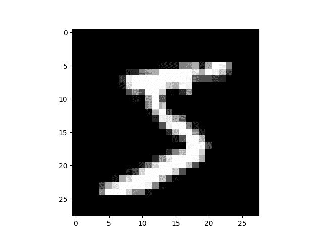
每个图像是 28 x 28，被存储为长度为 784（=28x28）的扁平化行。让我们看一个；我们需要先将其重塑为 2D。

from matplotlib import pyplot
import numpy as nppyplot.imshow(x_train[0].reshape((28, 28)), cmap="gray")
# ``pyplot.show()`` only if not on Colab
try:import google.colab
except ImportError:pyplot.show()
print(x_train.shape) 

(50000, 784) 

PyTorch 使用torch.tensor，而不是 numpy 数组，所以我们需要转换我们的数据。

import torchx_train, y_train, x_valid, y_valid = map(torch.tensor, (x_train, y_train, x_valid, y_valid)
)
n, c = x_train.shape
print(x_train, y_train)
print(x_train.shape)
print(y_train.min(), y_train.max()) 

tensor([[0., 0., 0.,  ..., 0., 0., 0.],[0., 0., 0.,  ..., 0., 0., 0.],[0., 0., 0.,  ..., 0., 0., 0.],...,[0., 0., 0.,  ..., 0., 0., 0.],[0., 0., 0.,  ..., 0., 0., 0.],[0., 0., 0.,  ..., 0., 0., 0.]]) tensor([5, 0, 4,  ..., 8, 4, 8])
torch.Size([50000, 784])
tensor(0) tensor(9) 

从头开始构建神经网络（不使用torch.nn）

让我们首先使用纯粹的 PyTorch 张量操作创建一个模型。我们假设您已经熟悉神经网络的基础知识。（如果您不熟悉，您可以在course.fast.ai学习）。

PyTorch 提供了创建随机或零填充张量的方法，我们将使用它们来创建简单线性模型的权重和偏置。这些只是常规张量，但有一个非常特殊的附加功能：我们告诉 PyTorch 它们需要梯度。这会导致 PyTorch 记录在张量上执行的所有操作，以便在反向传播期间自动计算梯度！

对于权重，我们在初始化之后设置requires_grad，因为我们不希望该步骤包含在梯度中。（请注意，PyTorch 中的下划线_表示该操作是原地执行的。）

注意

我们在这里使用Xavier 初始化来初始化权重（通过乘以1/sqrt(n)）。

import mathweights = torch.randn(784, 10) / math.sqrt(784)
weights.requires_grad_()
bias = torch.zeros(10, requires_grad=True) 

由于 PyTorch 能够自动计算梯度，我们可以使用任何标准的 Python 函数（或可调用对象）作为模型！因此，让我们只需编写一个简单的矩阵乘法和广播加法来创建一个简单的线性模型。我们还需要一个激活函数，所以我们将编写 log_softmax 并使用它。请记住：尽管 PyTorch 提供了许多预先编写的损失函数、激活函数等，但您可以轻松使用纯 Python 编写自己的函数。PyTorch 甚至会自动为您的函数创建快速的 GPU 或矢量化 CPU 代码。

def log_softmax(x):return x - x.exp().sum(-1).log().unsqueeze(-1)def model(xb):return log_softmax(xb @ weights + bias) 

在上面，@代表矩阵乘法运算。我们将在一批数据（在本例中为 64 张图像）上调用我们的函数。这是一个前向传递。请注意，在这个阶段我们的预测不会比随机更好，因为我们从随机权重开始。

bs = 64  # batch sizexb = x_train[0:bs]  # a mini-batch from x
preds = model(xb)  # predictions
preds[0], preds.shape
print(preds[0], preds.shape) 

tensor([-2.5452, -2.0790, -2.1832, -2.6221, -2.3670, -2.3854, -2.9432, -2.4391,-1.8657, -2.0355], grad_fn=<SelectBackward0>) torch.Size([64, 10]) 

正如您所看到的，preds张量不仅包含张量值，还包含一个梯度函数。我们稍后将使用这个函数进行反向传播。

让我们实现负对数似然作为损失函数（同样，我们可以直接使用标准的 Python）：

def nll(input, target):return -input[range(target.shape[0]), target].mean()loss_func = nll 

让我们检查我们的随机模型的损失，这样我们就可以看到在后续的反向传播过程中是否有改善。

yb = y_train[0:bs]
print(loss_func(preds, yb)) 

tensor(2.4020, grad_fn=<NegBackward0>) 

让我们还实现一个函数来计算模型的准确性。对于每个预测，如果具有最大值的索引与目标值匹配，则预测是正确的。

def accuracy(out, yb):preds = torch.argmax(out, dim=1)return (preds == yb).float().mean() 

让我们检查我们的随机模型的准确性，这样我们就可以看到随着损失的改善，我们的准确性是否也在提高。

print(accuracy(preds, yb)) 

tensor(0.0938) 

现在我们可以运行训练循环。对于每次迭代，我们将：

• 选择一个大小为bs的数据小批量

• 使用模型进行预测

• 计算损失

• loss.backward()更新模型的梯度，在这种情况下是weights和bias。

现在我们使用这些梯度来更新权重和偏置。我们在torch.no_grad()上下文管理器中执行此操作，因为我们不希望这些操作被记录下来用于下一次计算梯度。您可以在这里关于 PyTorch 的 Autograd 如何记录操作的信息。

然后我们将梯度设置为零，这样我们就准备好进行下一次循环。否则，我们的梯度会记录所有已发生的操作的累计总数（即loss.backward() 添加梯度到已经存储的内容，而不是替换它们）。

提示

您可以使用标准的 Python 调试器逐步执行 PyTorch 代码，从而可以在每个步骤检查各种变量的值。取消下面的set_trace()注释以尝试。

from IPython.core.debugger import set_tracelr = 0.5  # learning rate
epochs = 2  # how many epochs to train forfor epoch in range(epochs):for i in range((n - 1) // bs + 1):#         set_trace()start_i = i * bsend_i = start_i + bsxb = x_train[start_i:end_i]yb = y_train[start_i:end_i]pred = model(xb)loss = loss_func(pred, yb)loss.backward()with torch.no_grad():weights -= weights.grad * lrbias -= bias.grad * lrweights.grad.zero_()bias.grad.zero_() 

就是这样：我们已经从头开始创建和训练了一个最小的神经网络（在这种情况下，是一个逻辑回归，因为我们没有隐藏层）！

让我们检查损失和准确性，并将其与之前的结果进行比较。我们预计损失会减少，准确性会增加，事实也是如此。

print(loss_func(model(xb), yb), accuracy(model(xb), yb)) 

tensor(0.0813, grad_fn=<NegBackward0>) tensor(1.) 

使用torch.nn.functional

现在我们将重构我们的代码，使其与以前的代码执行相同的操作，只是我们将开始利用 PyTorch 的nn类使其更简洁和灵活。从这里开始的每一步，我们应该使我们的代码更短、更易理解和/或更灵活。

第一个最简单的步骤是通过用torch.nn.functional中的函数替换我们手写的激活和损失函数来缩短我们的代码（通常按照惯例，这个模块被导入到F命名空间中）。该模块包含torch.nn库中的所有函数（而库的其他部分包含类）。除了各种损失和激活函数外，您还会在这里找到一些方便创建神经网络的函数，如池化函数。（还有用于执行卷积、线性层等操作的函数，但正如我们将看到的，这些通常更好地使用库的其他部分处理。）

如果您使用负对数似然损失和对数 softmax 激活函数，那么 Pytorch 提供了一个结合了两者的单个函数F.cross_entropy。因此，我们甚至可以从我们的模型中删除激活函数。

import torch.nn.functional as Floss_func = F.cross_entropydef model(xb):return xb @ weights + bias 

请注意，在model函数中我们不再调用log_softmax。让我们确认我们的损失和准确率与以前相同：

print(loss_func(model(xb), yb), accuracy(model(xb), yb)) 

tensor(0.0813, grad_fn=<NllLossBackward0>) tensor(1.) 

使用nn.Module进行重构

接下来，我们将使用nn.Module和nn.Parameter，以获得更清晰、更简洁的训练循环。我们子类化nn.Module（它本身是一个类，能够跟踪状态）。在这种情况下，我们想要创建一个类来保存我们的权重、偏置和前向步骤的方法。nn.Module有许多属性和方法（如.parameters()和.zero_grad()），我们将使用它们。

注意

nn.Module（大写 M）是 PyTorch 特定的概念，是一个我们将经常使用的类。nn.Module不应与 Python 概念中的（小写 m）模块混淆，后者是一个可以被导入的 Python 代码文件。

from torch import nnclass Mnist_Logistic(nn.Module):def __init__(self):super().__init__()self.weights = nn.Parameter(torch.randn(784, 10) / math.sqrt(784))self.bias = nn.Parameter(torch.zeros(10))def forward(self, xb):return xb @ self.weights + self.bias 

由于我们现在使用的是对象而不仅仅是函数，我们首先要实例化我们的模型：

model = Mnist_Logistic() 

现在我们可以像以前一样计算损失。请注意，nn.Module对象被用作函数（即它们是可调用的），但在幕后，Pytorch 会自动调用我们的forward方法。

print(loss_func(model(xb), yb)) 

tensor(2.3096, grad_fn=<NllLossBackward0>) 

以前在我们的训练循环中，我们必须按名称更新每个参数的值，并手动将每个参数的梯度归零，就像这样：

with torch.no_grad():weights -= weights.grad * lrbias -= bias.grad * lrweights.grad.zero_()bias.grad.zero_() 

现在我们可以利用 model.parameters()和 model.zero_grad()（这两者都由 PyTorch 为nn.Module定义）来使这些步骤更简洁，更不容易出错，特别是如果我们有一个更复杂的模型：

with torch.no_grad():for p in model.parameters(): p -= p.grad * lrmodel.zero_grad() 

我们将把我们的小训练循环封装在一个fit函数中，以便以后可以再次运行它。

def fit():for epoch in range(epochs):for i in range((n - 1) // bs + 1):start_i = i * bsend_i = start_i + bsxb = x_train[start_i:end_i]yb = y_train[start_i:end_i]pred = model(xb)loss = loss_func(pred, yb)loss.backward()with torch.no_grad():for p in model.parameters():p -= p.grad * lrmodel.zero_grad()fit() 

让我们再次确认我们的损失是否下降了：

print(loss_func(model(xb), yb)) 

tensor(0.0821, grad_fn=<NllLossBackward0>) 

使用nn.Linear进行重构

我们继续重构我们的代码。我们将使用 Pytorch 类nn.Linear来代替手动定义和初始化self.weights和self.bias，以及计算xb @ self.weights + self.bias，这个线性层会为我们完成所有这些工作。Pytorch 有许多预定义的层类型，可以极大简化我们的代码，而且通常也会使其更快。

class Mnist_Logistic(nn.Module):def __init__(self):super().__init__()self.lin = nn.Linear(784, 10)def forward(self, xb):return self.lin(xb) 

我们实例化我们的模型，并像以前一样计算损失：

model = Mnist_Logistic()
print(loss_func(model(xb), yb)) 

tensor(2.3313, grad_fn=<NllLossBackward0>) 

我们仍然可以像以前一样使用我们的fit方法。

fit()print(loss_func(model(xb), yb)) 

tensor(0.0819, grad_fn=<NllLossBackward0>) 

使用torch.optim进行重构

Pytorch 还有一个包含各种优化算法的包，torch.optim。我们可以使用优化器的step方法来进行前向步骤，而不是手动更新每个参数。

这将使我们能够替换以前手动编码的优化步骤：

with torch.no_grad():for p in model.parameters(): p -= p.grad * lrmodel.zero_grad() 

而是使用：

opt.step()
opt.zero_grad() 

（optim.zero_grad()将梯度重置为 0，我们需要在计算下一个小批量的梯度之前调用它。）

from torch import optim 

我们将定义一个小函数来创建我们的模型和优化器，以便将来可以重复使用它。

def get_model():model = Mnist_Logistic()return model, optim.SGD(model.parameters(), lr=lr)model, opt = get_model()
print(loss_func(model(xb), yb))for epoch in range(epochs):for i in range((n - 1) // bs + 1):start_i = i * bsend_i = start_i + bsxb = x_train[start_i:end_i]yb = y_train[start_i:end_i]pred = model(xb)loss = loss_func(pred, yb)loss.backward()opt.step()opt.zero_grad()print(loss_func(model(xb), yb)) 

tensor(2.2659, grad_fn=<NllLossBackward0>)
tensor(0.0810, grad_fn=<NllLossBackward0>) 

使用 Dataset 进行重构

PyTorch 有一个抽象的 Dataset 类。一个 Dataset 可以是任何具有__len__函数（由 Python 的标准len函数调用）和__getitem__函数作为索引方式的东西。这个教程演示了创建一个自定义的FacialLandmarkDataset类作为Dataset子类的一个很好的例子。

PyTorch 的TensorDataset是一个包装张量的数据集。通过定义长度和索引方式，这也为我们提供了一种在张量的第一维度上进行迭代、索引和切片的方式。这将使我们更容易在训练时同时访问独立变量和因变量。

from torch.utils.data import TensorDataset 

x_train和y_train可以合并在一个TensorDataset中，这样在迭代和切片时会更容易。

train_ds = TensorDataset(x_train, y_train) 

以前，我们必须分别迭代x和y值的小批次：

xb = x_train[start_i:end_i]
yb = y_train[start_i:end_i] 

现在，我们可以一起完成这两个步骤：

xb,yb = train_ds[i*bs : i*bs+bs] 

model, opt = get_model()for epoch in range(epochs):for i in range((n - 1) // bs + 1):xb, yb = train_ds[i * bs: i * bs + bs]pred = model(xb)loss = loss_func(pred, yb)loss.backward()opt.step()opt.zero_grad()print(loss_func(model(xb), yb)) 

tensor(0.0826, grad_fn=<NllLossBackward0>) 

使用DataLoader进行重构

PyTorch 的DataLoader负责管理批次。您可以从任何Dataset创建一个DataLoader。DataLoader使得批次迭代更容易。不需要使用train_ds[i*bs : i*bs+bs]，DataLoader会自动给我们每个小批次。

from torch.utils.data import DataLoadertrain_ds = TensorDataset(x_train, y_train)
train_dl = DataLoader(train_ds, batch_size=bs) 

以前，我们的循环像这样迭代批次(xb, yb)：

for i in range((n-1)//bs + 1):xb,yb = train_ds[i*bs : i*bs+bs]pred = model(xb) 

现在，我们的循环更加清晰，因为(xb, yb)会自动从数据加载器中加载：

for xb,yb in train_dl:pred = model(xb) 

model, opt = get_model()for epoch in range(epochs):for xb, yb in train_dl:pred = model(xb)loss = loss_func(pred, yb)loss.backward()opt.step()opt.zero_grad()print(loss_func(model(xb), yb)) 

tensor(0.0818, grad_fn=<NllLossBackward0>) 

由于 PyTorch 的nn.Module、nn.Parameter、Dataset和DataLoader，我们的训练循环现在变得更小更容易理解。现在让我们尝试添加创建有效模型所需的基本特性。

添加验证

在第 1 节中，我们只是试图建立一个合理的训练循环来用于训练数据。实际上，您总是应该有一个验证集，以便确定是否过拟合。

对训练数据进行洗牌是重要的，以防止批次之间的相关性和过拟合。另一方面，验证损失无论我们是否对验证集进行洗牌都是相同的。由于洗牌需要额外的时间，对验证数据进行洗牌是没有意义的。

我们将使用验证集的批量大小是训练集的两倍。这是因为验证集不需要反向传播，因此占用的内存较少（不需要存储梯度）。我们利用这一点使用更大的批量大小更快地计算损失。

train_ds = TensorDataset(x_train, y_train)
train_dl = DataLoader(train_ds, batch_size=bs, shuffle=True)valid_ds = TensorDataset(x_valid, y_valid)
valid_dl = DataLoader(valid_ds, batch_size=bs * 2) 

我们将在每个 epoch 结束时计算并打印验证损失。

（请注意，在训练之前我们总是调用model.train()，在推理之前我们总是调用model.eval()，因为这些被nn.BatchNorm2d和nn.Dropout等层使用以确保这些不同阶段的适当行为。）

model, opt = get_model()for epoch in range(epochs):model.train()for xb, yb in train_dl:pred = model(xb)loss = loss_func(pred, yb)loss.backward()opt.step()opt.zero_grad()model.eval()with torch.no_grad():valid_loss = sum(loss_func(model(xb), yb) for xb, yb in valid_dl)print(epoch, valid_loss / len(valid_dl)) 

0 tensor(0.3048)
1 tensor(0.2872) 

创建 fit()和 get_data()

现在我们将进行一些重构。由于我们两次都要计算训练集和验证集的损失，让我们将其制作成自己的函数loss_batch，用于计算一个 batch 的损失。

我们为训练集传入一个优化器，并用它执行反向传播。对于验证集，我们不传入优化器，所以该方法不执行反向传播。

def loss_batch(model, loss_func, xb, yb, opt=None):loss = loss_func(model(xb), yb)if opt is not None:loss.backward()opt.step()opt.zero_grad()return loss.item(), len(xb) 

fit运行必要的操作来训练我们的模型，并计算每个 epoch 的训练和验证损失。

import numpy as npdef fit(epochs, model, loss_func, opt, train_dl, valid_dl):for epoch in range(epochs):model.train()for xb, yb in train_dl:loss_batch(model, loss_func, xb, yb, opt)model.eval()with torch.no_grad():losses, nums = zip(*[loss_batch(model, loss_func, xb, yb) for xb, yb in valid_dl])val_loss = np.sum(np.multiply(losses, nums)) / np.sum(nums)print(epoch, val_loss) 

get_data返回训练集和验证集的数据加载器。

def get_data(train_ds, valid_ds, bs):return (DataLoader(train_ds, batch_size=bs, shuffle=True),DataLoader(valid_ds, batch_size=bs * 2),) 

现在，我们整个获取数据加载器和拟合模型的过程可以在 3 行代码中运行：

train_dl, valid_dl = get_data(train_ds, valid_ds, bs)
model, opt = get_model()
fit(epochs, model, loss_func, opt, train_dl, valid_dl) 

0 0.2939354367017746
1 0.3258970756947994 

您可以使用这基本的 3 行代码来训练各种模型。让我们看看是否可以使用它们来训练卷积神经网络（CNN）！

切换到 CNN

现在我们将建立一个具有三个卷积层的神经网络。由于上一节中的函数都不假设模型形式，我们将能够使用它们来训练 CNN 而无需任何修改。

我们将使用 PyTorch 预定义的Conv2d类作为我们的卷积层。我们定义了一个具有 3 个卷积层的 CNN。每个卷积后面跟着一个 ReLU。最后，我们执行平均池化。（注意view是 PyTorch 版本的 Numpy 的reshape）

class Mnist_CNN(nn.Module):def __init__(self):super().__init__()self.conv1 = nn.Conv2d(1, 16, kernel_size=3, stride=2, padding=1)self.conv2 = nn.Conv2d(16, 16, kernel_size=3, stride=2, padding=1)self.conv3 = nn.Conv2d(16, 10, kernel_size=3, stride=2, padding=1)def forward(self, xb):xb = xb.view(-1, 1, 28, 28)xb = F.relu(self.conv1(xb))xb = F.relu(self.conv2(xb))xb = F.relu(self.conv3(xb))xb = F.avg_pool2d(xb, 4)return xb.view(-1, xb.size(1))lr = 0.1 

动量是随机梯度下降的一种变体，它考虑了先前的更新，通常导致更快的训练。

model = Mnist_CNN()
opt = optim.SGD(model.parameters(), lr=lr, momentum=0.9)fit(epochs, model, loss_func, opt, train_dl, valid_dl) 

0 0.35247018008232117
1 0.25782823679447175 

使用nn.Sequential

torch.nn还有另一个方便的类，我们可以用它来简化我们的代码：Sequential。Sequential对象按顺序运行其中包含的每个模块。这是编写我们的神经网络的一种更简单的方法。

为了利用这一点，我们需要能够轻松地从给定函数定义一个自定义层。例如，PyTorch 没有一个视图层，我们需要为我们的网络创建一个。Lambda将创建一个层，然后我们可以在使用Sequential定义网络时使用它。

class Lambda(nn.Module):def __init__(self, func):super().__init__()self.func = funcdef forward(self, x):return self.func(x)def preprocess(x):return x.view(-1, 1, 28, 28) 

使用Sequential创建的模型很简单：

model = nn.Sequential(Lambda(preprocess),nn.Conv2d(1, 16, kernel_size=3, stride=2, padding=1),nn.ReLU(),nn.Conv2d(16, 16, kernel_size=3, stride=2, padding=1),nn.ReLU(),nn.Conv2d(16, 10, kernel_size=3, stride=2, padding=1),nn.ReLU(),nn.AvgPool2d(4),Lambda(lambda x: x.view(x.size(0), -1)),
)opt = optim.SGD(model.parameters(), lr=lr, momentum=0.9)fit(epochs, model, loss_func, opt, train_dl, valid_dl) 

0 0.3226209937572479
1 0.2234949318766594 

包装DataLoader

我们的 CNN 相当简洁，但只适用于 MNIST，因为：

• 它假设输入是一个 28*28 的长向量

• 它假设最终的 CNN 网格大小为 4*4（因为这是我们使用的平均池化核大小）

让我们摆脱这两个假设，这样我们的模型就可以处理任何 2D 单通道图像。首先，我们可以通过将数据预处理移入生成器来删除初始的 Lambda 层：

def preprocess(x, y):return x.view(-1, 1, 28, 28), yclass WrappedDataLoader:def __init__(self, dl, func):self.dl = dlself.func = funcdef __len__(self):return len(self.dl)def __iter__(self):for b in self.dl:yield (self.func(*b))train_dl, valid_dl = get_data(train_ds, valid_ds, bs)
train_dl = WrappedDataLoader(train_dl, preprocess)
valid_dl = WrappedDataLoader(valid_dl, preprocess) 

接下来，我们可以用nn.AdaptiveAvgPool2d替换nn.AvgPool2d，这样我们可以定义我们想要的输出张量的大小，而不是我们拥有的输入张量。因此，我们的模型将适用于任何大小的输入。

model = nn.Sequential(nn.Conv2d(1, 16, kernel_size=3, stride=2, padding=1),nn.ReLU(),nn.Conv2d(16, 16, kernel_size=3, stride=2, padding=1),nn.ReLU(),nn.Conv2d(16, 10, kernel_size=3, stride=2, padding=1),nn.ReLU(),nn.AdaptiveAvgPool2d(1),Lambda(lambda x: x.view(x.size(0), -1)),
)opt = optim.SGD(model.parameters(), lr=lr, momentum=0.9) 

让我们试一试：

fit(epochs, model, loss_func, opt, train_dl, valid_dl) 

0 0.3148617018699646
1 0.20678156037330628 

使用您的 GPU

如果您有幸拥有支持 CUDA 的 GPU（您可以从大多数云提供商租用一个约 0.50 美元/小时），您可以使用它加速您的代码。首先检查您的 GPU 在 Pytorch 中是否正常工作：

print(torch.cuda.is_available()) 

True 

然后为其创建一个设备对象：

dev = torch.device("cuda") if torch.cuda.is_available() else torch.device("cpu") 

让我们更新preprocess以将批次移动到 GPU：

def preprocess(x, y):return x.view(-1, 1, 28, 28).to(dev), y.to(dev)train_dl, valid_dl = get_data(train_ds, valid_ds, bs)
train_dl = WrappedDataLoader(train_dl, preprocess)
valid_dl = WrappedDataLoader(valid_dl, preprocess) 

最后，我们可以将我们的模型移动到 GPU 上。

model.to(dev)
opt = optim.SGD(model.parameters(), lr=lr, momentum=0.9) 

您应该发现现在运行得更快了：

fit(epochs, model, loss_func, opt, train_dl, valid_dl) 

0 0.17924857176542283
1 0.17124842552542688 

结束思考

现在我们有一个通用的数据管道和训练循环，您可以使用它来训练许多类型的模型使用 Pytorch。要了解现在训练模型有多简单，请查看mnist_sample 笔记本。

当然，您可能想要添加许多其他功能，例如数据增强、超参数调整、监视训练、迁移学习等。这些功能在 fastai 库中可用，该库是使用本教程中展示的相同设计方法开发的，为希望进一步发展其模型的从业者提供了一个自然的下一步。

我们在本教程开始时承诺通过示例解释每个torch.nn，torch.optim，Dataset和DataLoader。所以让我们总结一下我们所看到的内容：

• torch.nn：
• • Module：创建一个可调用的函数，但也可以包含状态（例如神经网络层权重）。它知道它包含的Parameter(s)，可以将它们的梯度清零，循环遍历它们进行权重更新等。
  • Parameter：一个张量的包装器，告诉Module它有需要在反向传播过程中更新的权重。只有设置了 requires_grad 属性的张量才会被更新
  • functional：一个模块（通常按照惯例导入到F命名空间中），其中包含激活函数、损失函数等，以及卷积和线性层的非状态版本。
• torch.optim：包含诸如SGD之类的优化器，在反向步骤中更新Parameter的权重
• Dataset：具有__len__和__getitem__的对象的抽象接口，包括 Pytorch 提供的类，如TensorDataset
• DataLoader：接受任何Dataset并创建一个返回数据批次的迭代器。

脚本的总运行时间：（0 分钟 36.765 秒）

下载 Python 源代码：nn_tutorial.py

下载 Jupyter 笔记本：nn_tutorial.ipynb

Sphinx-Gallery 生成的画廊

使用 TensorBoard 可视化模型、数据和训练

原文：pytorch.org/tutorials/intermediate/tensorboard_tutorial.html

译者：飞龙

协议：CC BY-NC-SA 4.0

在60 分钟入门中，我们向您展示如何加载数据，将其通过我们定义的nn.Module子类模型，对训练数据进行训练，并在测试数据上进行测试。为了了解发生了什么，我们在模型训练时打印出一些统计数据，以了解训练是否在进行中。然而，我们可以做得更好：PyTorch 集成了 TensorBoard，这是一个用于可视化神经网络训练结果的工具。本教程演示了一些其功能，使用Fashion-MNIST 数据集，可以使用 torchvision.datasets 将其读入 PyTorch。

在本教程中，我们将学习如何：

1. 读取数据并进行适当的转换（与之前的教程几乎相同）。
3. 设置 TensorBoard。
5. 写入 TensorBoard。
7. 使用 TensorBoard 检查模型架构。
9. 使用 TensorBoard 创建上一个教程中创建的可视化的交互版本，代码更少

具体来说，在第 5 点上，我们将看到：

• 检查我们的训练数据的几种方法
• 如何在模型训练过程中跟踪我们模型的性能
• 如何评估我们模型训练后的性能。

我们将从CIFAR-10 教程中类似的样板代码开始：

# imports
import matplotlib.pyplot as plt
import numpy as npimport torch
import torchvision
import torchvision.transforms as transformsimport torch.nn as nn
import torch.nn.functional as F
import torch.optim as optim# transforms
transform = transforms.Compose([transforms.ToTensor(),transforms.Normalize((0.5,), (0.5,))])# datasets
trainset = torchvision.datasets.FashionMNIST('./data',download=True,train=True,transform=transform)
testset = torchvision.datasets.FashionMNIST('./data',download=True,train=False,transform=transform)# dataloaders
trainloader = torch.utils.data.DataLoader(trainset, batch_size=4,shuffle=True, num_workers=2)testloader = torch.utils.data.DataLoader(testset, batch_size=4,shuffle=False, num_workers=2)# constant for classes
classes = ('T-shirt/top', 'Trouser', 'Pullover', 'Dress', 'Coat','Sandal', 'Shirt', 'Sneaker', 'Bag', 'Ankle Boot')# helper function to show an image
# (used in the `plot_classes_preds` function below)
def matplotlib_imshow(img, one_channel=False):if one_channel:img = img.mean(dim=0)img = img / 2 + 0.5     # unnormalizenpimg = img.numpy()if one_channel:plt.imshow(npimg, cmap="Greys")else:plt.imshow(np.transpose(npimg, (1, 2, 0))) 

我们将定义一个类似于该教程的模型架构，只需进行轻微修改以适应图像现在是单通道而不是三通道，28x28 而不是 32x32 的事实：

class Net(nn.Module):def __init__(self):super(Net, self).__init__()self.conv1 = nn.Conv2d(1, 6, 5)self.pool = nn.MaxPool2d(2, 2)self.conv2 = nn.Conv2d(6, 16, 5)self.fc1 = nn.Linear(16 * 4 * 4, 120)self.fc2 = nn.Linear(120, 84)self.fc3 = nn.Linear(84, 10)def forward(self, x):x = self.pool(F.relu(self.conv1(x)))x = self.pool(F.relu(self.conv2(x)))x = x.view(-1, 16 * 4 * 4)x = F.relu(self.fc1(x))x = F.relu(self.fc2(x))x = self.fc3(x)return xnet = Net() 

我们将从之前定义的相同的optimizer和criterion开始：

criterion = nn.CrossEntropyLoss()
optimizer = optim.SGD(net.parameters(), lr=0.001, momentum=0.9) 

1. TensorBoard 设置

现在我们将设置 TensorBoard，从torch.utils导入tensorboard并定义一个SummaryWriter，这是我们向 TensorBoard 写入信息的关键对象。

from torch.utils.tensorboard import SummaryWriter# default `log_dir` is "runs" - we'll be more specific here
writer = SummaryWriter('runs/fashion_mnist_experiment_1') 

请注意，这一行代码会创建一个runs/fashion_mnist_experiment_1文件夹。

2. 写入 TensorBoard

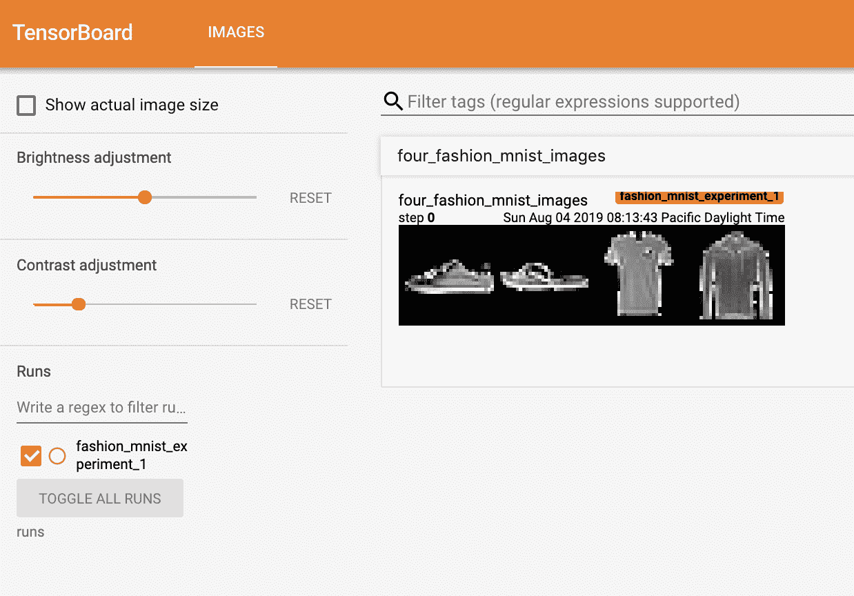
现在让我们向 TensorBoard 写入一张图片 - 具体来说，使用make_grid创建一个网格。

# get some random training images
dataiter = iter(trainloader)
images, labels = next(dataiter)# create grid of images
img_grid = torchvision.utils.make_grid(images)# show images
matplotlib_imshow(img_grid, one_channel=True)# write to tensorboard
writer.add_image('four_fashion_mnist_images', img_grid) 

现在正在运行

tensorboard --logdir=runs 

从命令行中导航到localhost:6006应该显示以下内容。

现在你知道如何使用 TensorBoard 了！然而，这个例子也可以在 Jupyter Notebook 中完成 - TensorBoard 真正擅长的是创建交互式可视化。我们将在教程结束时介绍其中的一个，以及更多其他功能。

3. 使用 TensorBoard 检查模型

TensorBoard 的一个优势是它能够可视化复杂的模型结构。让我们可视化我们构建的模型。

writer.add_graph(net, images)
writer.close() 

现在刷新 TensorBoard 后，您应该看到一个类似于这样的“Graphs”选项卡：

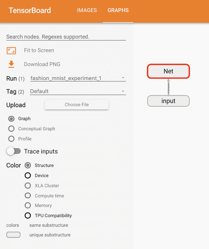
继续双击“Net”以展开，查看组成模型的各个操作的详细视图。

TensorBoard 有一个非常方便的功能，可以将高维数据（如图像数据）可视化为一个较低维度的空间；我们将在下面介绍这个功能。

4. 向 TensorBoard 添加“Projector”

我们可以通过add_embedding方法可视化高维数据的低维表示

# helper function
def select_n_random(data, labels, n=100):'''Selects n random datapoints and their corresponding labels from a dataset'''assert len(data) == len(labels)perm = torch.randperm(len(data))return data[perm][:n], labels[perm][:n]# select random images and their target indices
images, labels = select_n_random(trainset.data, trainset.targets)# get the class labels for each image
class_labels = [classes[lab] for lab in labels]# log embeddings
features = images.view(-1, 28 * 28)
writer.add_embedding(features,metadata=class_labels,label_img=images.unsqueeze(1))
writer.close() 

现在在 TensorBoard 的“Projector”标签中，您可以看到这 100 张图片 - 每张图片都是 784 维的 - 投影到三维空间中。此外，这是交互式的：您可以单击并拖动以旋转三维投影。最后，为了使可视化更容易看到，有几个提示：在左上角选择“颜色：标签”，并启用“夜间模式”，这将使图像更容易看到，因为它们的背景是白色的：

现在我们已经彻底检查了我们的数据，让我们展示一下 TensorBoard 如何使跟踪模型训练和评估更清晰，从训练开始。

5. 使用 TensorBoard 跟踪模型训练

在先前的示例中，我们只是打印了模型的运行损失，每 2000 次迭代一次。现在，我们将把运行损失记录到 TensorBoard 中，以及通过plot_classes_preds函数查看模型的预测。

# helper functionsdef images_to_probs(net, images):'''Generates predictions and corresponding probabilities from a trainednetwork and a list of images'''output = net(images)# convert output probabilities to predicted class_, preds_tensor = torch.max(output, 1)preds = np.squeeze(preds_tensor.numpy())return preds, [F.softmax(el, dim=0)[i].item() for i, el in zip(preds, output)]def plot_classes_preds(net, images, labels):'''Generates matplotlib Figure using a trained network, along with imagesand labels from a batch, that shows the network's top prediction alongwith its probability, alongside the actual label, coloring thisinformation based on whether the prediction was correct or not.Uses the "images_to_probs" function.'''preds, probs = images_to_probs(net, images)# plot the images in the batch, along with predicted and true labelsfig = plt.figure(figsize=(12, 48))for idx in np.arange(4):ax = fig.add_subplot(1, 4, idx+1, xticks=[], yticks=[])matplotlib_imshow(images[idx], one_channel=True)ax.set_title("{0}, {1:.1f}%\n(label: {2})".format(classes[preds[idx]],probs[idx] * 100.0,classes[labels[idx]]),color=("green" if preds[idx]==labels[idx].item() else "red"))return fig 

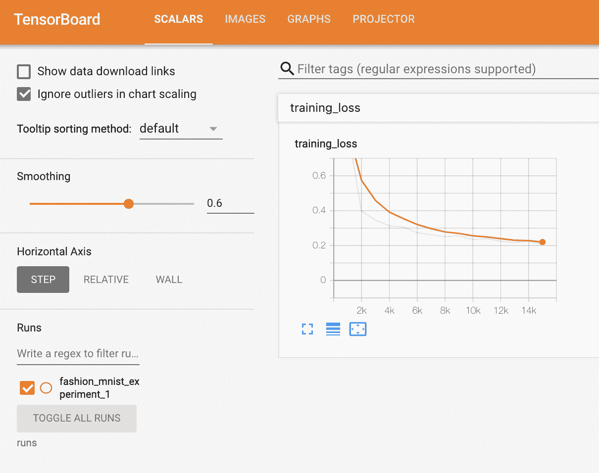
最后，让我们使用之前教程中相同的模型训练代码来训练模型，但是每 1000 批次将结果写入 TensorBoard，而不是打印到控制台；这可以使用add_scalar函数来实现。

此外，当我们训练时，我们将生成一幅图像，显示模型对该批次中包含的四幅图像的预测与实际结果。

running_loss = 0.0
for epoch in range(1):  # loop over the dataset multiple timesfor i, data in enumerate(trainloader, 0):# get the inputs; data is a list of [inputs, labels]inputs, labels = data# zero the parameter gradientsoptimizer.zero_grad()# forward + backward + optimizeoutputs = net(inputs)loss = criterion(outputs, labels)loss.backward()optimizer.step()running_loss += loss.item()if i % 1000 == 999:    # every 1000 mini-batches...# ...log the running losswriter.add_scalar('training loss',running_loss / 1000,epoch * len(trainloader) + i)# ...log a Matplotlib Figure showing the model's predictions on a# random mini-batchwriter.add_figure('predictions vs. actuals',plot_classes_preds(net, inputs, labels),global_step=epoch * len(trainloader) + i)running_loss = 0.0
print('Finished Training') 

您现在可以查看标量标签，看看在训练的 15000 次迭代中绘制的运行损失：

此外，我们可以查看模型在学习过程中对任意批次的预测。查看“Images”标签，并在“预测与实际”可视化下滚动，以查看这一点；这向我们展示，例如，在仅 3000 次训练迭代后，模型已经能够区分视觉上不同的类别，如衬衫、运动鞋和外套，尽管它在训练后期变得更加自信：

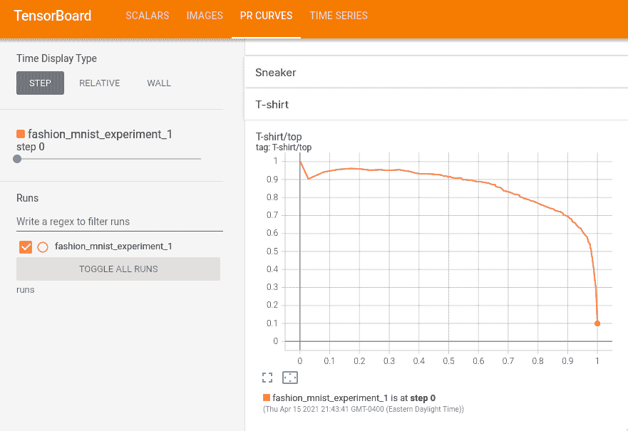
在之前的教程中，我们在模型训练后查看了每个类别的准确率；在这里，我们将使用 TensorBoard 来为每个类别绘制精确度-召回率曲线（好的解释在这里）。

6. 使用 TensorBoard 评估训练好的模型

# 1\. gets the probability predictions in a test_size x num_classes Tensor
# 2\. gets the preds in a test_size Tensor
# takes ~10 seconds to run
class_probs = []
class_label = []
with torch.no_grad():for data in testloader:images, labels = dataoutput = net(images)class_probs_batch = [F.softmax(el, dim=0) for el in output]class_probs.append(class_probs_batch)class_label.append(labels)test_probs = torch.cat([torch.stack(batch) for batch in class_probs])
test_label = torch.cat(class_label)# helper function
def add_pr_curve_tensorboard(class_index, test_probs, test_label, global_step=0):'''Takes in a "class_index" from 0 to 9 and plots the correspondingprecision-recall curve'''tensorboard_truth = test_label == class_indextensorboard_probs = test_probs[:, class_index]writer.add_pr_curve(classes[class_index],tensorboard_truth,tensorboard_probs,global_step=global_step)writer.close()# plot all the pr curves
for i in range(len(classes)):add_pr_curve_tensorboard(i, test_probs, test_label) 

现在您将看到一个包含每个类别精确度-召回率曲线的“PR 曲线”标签。继续浏览；您会看到在某些类别上，模型几乎有 100%的“曲线下面积”，而在其他类别上，这个面积较低：

这就是 TensorBoard 和 PyTorch 与其集成的简介。当然，您可以在 Jupyter Notebook 中做 TensorBoard 所做的一切，但是使用 TensorBoard，您会得到默认情况下是交互式的可视化。

图像和视频

TorchVision 目标检测微调教程

原文：pytorch.org/tutorials/intermediate/torchvision_tutorial.html

译者：飞龙

协议：CC BY-NC-SA 4.0

注意

点击这里下载完整示例代码

在本教程中，我们将对宾夕法尼亚大学行人检测和分割数据库上的预训练Mask R-CNN模型进行微调。它包含 170 张图像，有 345 个行人实例，我们将用它来演示如何使用 torchvision 中的新功能来训练自定义数据集上的目标检测和实例分割模型。

注意

本教程仅适用于 torchvision 版本>=0.16 或夜间版本。如果您使用的是 torchvision<=0.15，请按照此教程操作。

定义数据集

用于训练目标检测、实例分割和人体关键点检测的参考脚本允许轻松支持添加新的自定义数据集。数据集应该继承自标准torch.utils.data.Dataset类，并实现__len__和__getitem__。

我们唯一要求的特定性是数据集__getitem__应返回一个元组：

• image：形状为[3, H, W]的torchvision.tv_tensors.Image，一个纯张量，或大小为(H, W)的 PIL 图像

• 目标：包含以下字段的字典

  • boxes，形状为[N, 4]的torchvision.tv_tensors.BoundingBoxes：N个边界框的坐标，格式为[x0, y0, x1, y1]，范围从0到W和0到H

  • labels，形状为[N]的整数torch.Tensor：每个边界框的标签。0始终表示背景类。

  • image_id，整数：图像标识符。它应该在数据集中的所有图像之间是唯一的，并在评估过程中使用

  • area，形状为[N]的浮点数torch.Tensor：边界框的面积。在使用 COCO 指标进行评估时使用，以区分小、中和大框之间的指标分数。

  • iscrowd，形状为[N]的 uint8 torch.Tensor：具有iscrowd=True的实例在评估过程中将被忽略。

  • （可选）masks，形状为[N, H, W]的torchvision.tv_tensors.Mask：每个对象的分割掩码

如果您的数据集符合上述要求，则可以在参考脚本中的训练和评估代码中使用。评估代码将使用pycocotools中的脚本，可以通过pip install pycocotools安装。

注意

对于 Windows，请使用以下命令从gautamchitnis安装pycocotools

pip install git+https://github.com/gautamchitnis/cocoapi.git@cocodataset-master#subdirectory=PythonAPI

关于labels的一点说明。模型将类0视为背景。如果您的数据集不包含背景类，则在labels中不应该有0。例如，假设您只有两类，猫和狗，您可以定义1（而不是0）表示猫，2表示狗。因此，例如，如果一张图像同时包含两类，则您的labels张量应该如下所示[1, 2]。

此外，如果您想在训练期间使用纵横比分组（以便每个批次只包含具有相似纵横比的图像），则建议还实现一个get_height_and_width方法，该方法返回图像的高度和宽度。如果未提供此方法，我们将通过__getitem__查询数据集的所有元素，这会将图像加载到内存中，比提供自定义方法慢。

为 PennFudan 编写自定义数据集

让我们为 PennFudan 数据集编写一个数据集。首先，让我们下载数据集并提取zip 文件：

wget https://www.cis.upenn.edu/~jshi/ped_html/PennFudanPed.zip -P data
cd data && unzip PennFudanPed.zip 

我们有以下文件夹结构：

PennFudanPed/PedMasks/FudanPed00001_mask.pngFudanPed00002_mask.pngFudanPed00003_mask.pngFudanPed00004_mask.png...PNGImages/FudanPed00001.pngFudanPed00002.pngFudanPed00003.pngFudanPed00004.png 

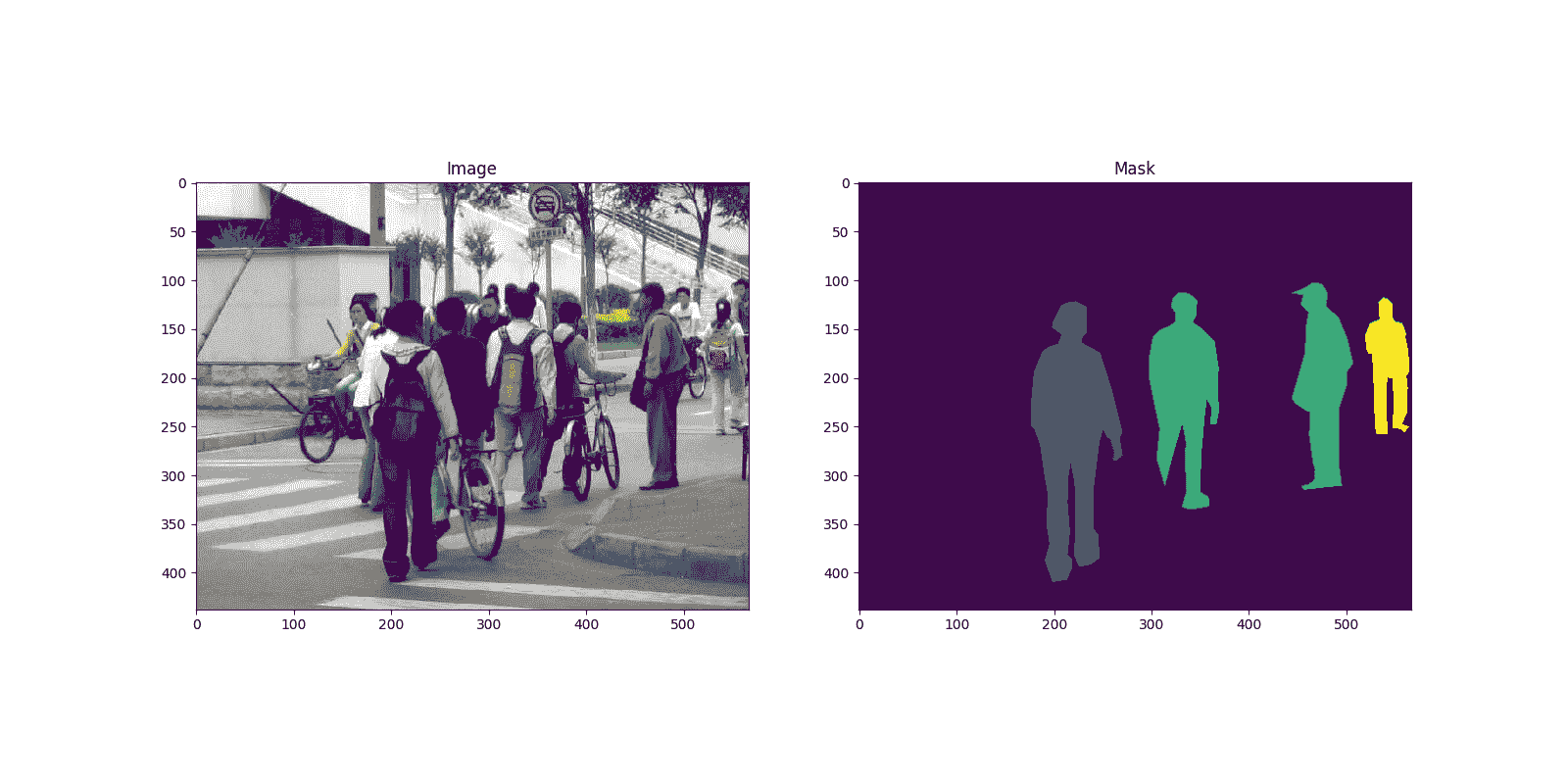
这是一对图像和分割蒙版的示例

import matplotlib.pyplot as plt
from torchvision.io import read_imageimage = read_image("data/PennFudanPed/PNGImages/FudanPed00046.png")
mask = read_image("data/PennFudanPed/PedMasks/FudanPed00046_mask.png")plt.figure(figsize=(16, 8))
plt.subplot(121)
plt.title("Image")
plt.imshow(image.permute(1, 2, 0))
plt.subplot(122)
plt.title("Mask")
plt.imshow(mask.permute(1, 2, 0)) 

<matplotlib.image.AxesImage object at 0x7f489920ffd0> 

因此，每个图像都有一个相应的分割蒙版，其中每种颜色对应不同的实例。让我们为这个数据集编写一个torch.utils.data.Dataset类。在下面的代码中，我们将图像、边界框和蒙版封装到torchvision.tv_tensors.TVTensor类中，以便我们能够应用 torchvision 内置的转换（新的转换 API）来完成给定的目标检测和分割任务。换句话说，图像张量将被torchvision.tv_tensors.Image封装，边界框将被封装为torchvision.tv_tensors.BoundingBoxes，蒙版将被封装为torchvision.tv_tensors.Mask。由于torchvision.tv_tensors.TVTensor是torch.Tensor的子类，封装的对象也是张量，并继承了普通的torch.Tensor API。有关 torchvision tv_tensors的更多信息，请参阅此文档。

import os
import torchfrom torchvision.io import read_image
from torchvision.ops.boxes import masks_to_boxes
from torchvision import tv_tensors
from torchvision.transforms.v2 import functional as Fclass PennFudanDataset(torch.utils.data.Dataset):def __init__(self, root, transforms):self.root = rootself.transforms = transforms# load all image files, sorting them to# ensure that they are alignedself.imgs = list(sorted(os.listdir(os.path.join(root, "PNGImages"))))self.masks = list(sorted(os.listdir(os.path.join(root, "PedMasks"))))def __getitem__(self, idx):# load images and masksimg_path = os.path.join(self.root, "PNGImages", self.imgs[idx])mask_path = os.path.join(self.root, "PedMasks", self.masks[idx])img = read_image(img_path)mask = read_image(mask_path)# instances are encoded as different colorsobj_ids = torch.unique(mask)# first id is the background, so remove itobj_ids = obj_ids[1:]num_objs = len(obj_ids)# split the color-encoded mask into a set# of binary masksmasks = (mask == obj_ids[:, None, None]).to(dtype=torch.uint8)# get bounding box coordinates for each maskboxes = masks_to_boxes(masks)# there is only one classlabels = torch.ones((num_objs,), dtype=torch.int64)image_id = idxarea = (boxes[:, 3] - boxes[:, 1]) * (boxes[:, 2] - boxes[:, 0])# suppose all instances are not crowdiscrowd = torch.zeros((num_objs,), dtype=torch.int64)# Wrap sample and targets into torchvision tv_tensors:img = tv_tensors.Image(img)target = {}target["boxes"] = tv_tensors.BoundingBoxes(boxes, format="XYXY", canvas_size=F.get_size(img))target["masks"] = tv_tensors.Mask(masks)target["labels"] = labelstarget["image_id"] = image_idtarget["area"] = areatarget["iscrowd"] = iscrowdif self.transforms is not None:img, target = self.transforms(img, target)return img, targetdef __len__(self):return len(self.imgs) 

这就是数据集的全部内容。现在让我们定义一个可以在此数据集上执行预测的模型。

定义您的模型

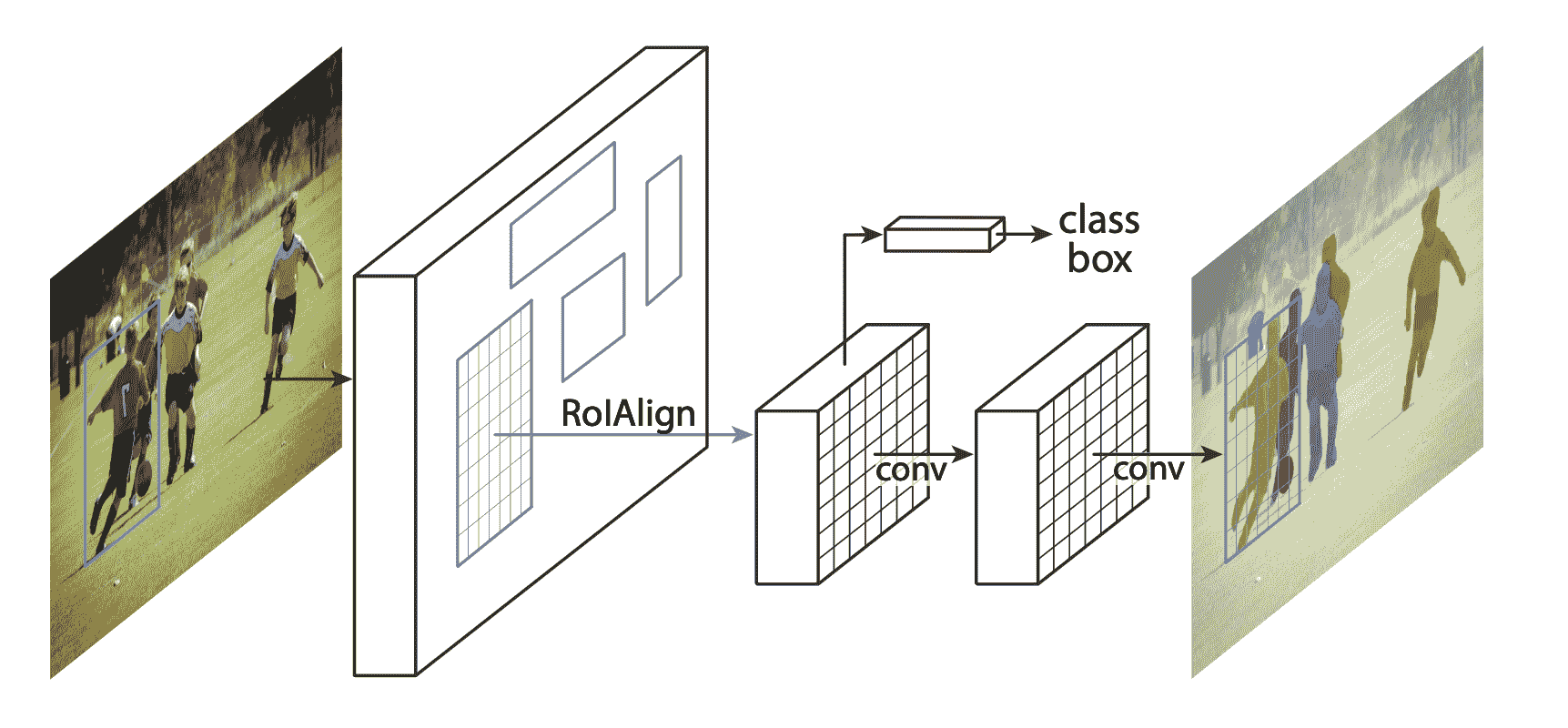
在本教程中，我们将使用基于Faster R-CNN的Mask R-CNN。Faster R-CNN 是一个模型，用于预测图像中潜在对象的边界框和类别分数。

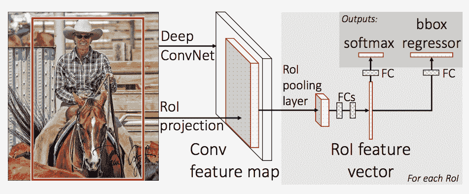
Mask R-CNN 在 Faster R-CNN 中添加了一个额外的分支，还为每个实例预测分割蒙版。

有两种常见情况可能需要修改 TorchVision Model Zoo 中的可用模型之一。第一种情况是当我们想要从预训练模型开始，只微调最后一层时。另一种情况是当我们想要用不同的主干替换模型的主干时（例如为了更快的预测）。

让我们看看在以下部分中我们将如何执行其中一个或另一个。

1 - 从预训练模型微调

假设您想从在 COCO 上预训练的模型开始，并希望对其进行微调以适应您的特定类别。以下是可能的操作方式：

import torchvision
from torchvision.models.detection.faster_rcnn import FastRCNNPredictor# load a model pre-trained on COCO
model = torchvision.models.detection.fasterrcnn_resnet50_fpn(weights="DEFAULT")# replace the classifier with a new one, that has
# num_classes which is user-defined
num_classes = 2  # 1 class (person) + background
# get number of input features for the classifier
in_features = model.roi_heads.box_predictor.cls_score.in_features
# replace the pre-trained head with a new one
model.roi_heads.box_predictor = FastRCNNPredictor(in_features, num_classes) 

Downloading: "https://download.pytorch.org/models/fasterrcnn_resnet50_fpn_coco-258fb6c6.pth" to /var/lib/jenkins/.cache/torch/hub/checkpoints/fasterrcnn_resnet50_fpn_coco-258fb6c6.pth0%|          | 0.00/160M [00:00<?, ?B/s]8%|7         | 12.1M/160M [00:00<00:01, 127MB/s]16%|#6        | 25.8M/160M [00:00<00:01, 137MB/s]25%|##4       | 39.6M/160M [00:00<00:00, 140MB/s]34%|###3      | 53.6M/160M [00:00<00:00, 143MB/s]42%|####2     | 67.5M/160M [00:00<00:00, 144MB/s]51%|#####     | 81.4M/160M [00:00<00:00, 145MB/s]60%|#####9    | 95.4M/160M [00:00<00:00, 145MB/s]68%|######8   | 109M/160M [00:00<00:00, 145MB/s]77%|#######7  | 123M/160M [00:00<00:00, 146MB/s]86%|########5 | 137M/160M [00:01<00:00, 146MB/s]95%|#########4| 151M/160M [00:01<00:00, 146MB/s]
100%|##########| 160M/160M [00:01<00:00, 144MB/s] 

2 - 修改模型以添加不同的主干

import torchvision
from torchvision.models.detection import FasterRCNN
from torchvision.models.detection.rpn import AnchorGenerator# load a pre-trained model for classification and return
# only the features
backbone = torchvision.models.mobilenet_v2(weights="DEFAULT").features
# ``FasterRCNN`` needs to know the number of
# output channels in a backbone. For mobilenet_v2, it's 1280
# so we need to add it here
backbone.out_channels = 1280# let's make the RPN generate 5 x 3 anchors per spatial
# location, with 5 different sizes and 3 different aspect
# ratios. We have a Tuple[Tuple[int]] because each feature
# map could potentially have different sizes and
# aspect ratios
anchor_generator = AnchorGenerator(sizes=((32, 64, 128, 256, 512),),aspect_ratios=((0.5, 1.0, 2.0),)
)# let's define what are the feature maps that we will
# use to perform the region of interest cropping, as well as
# the size of the crop after rescaling.
# if your backbone returns a Tensor, featmap_names is expected to
# be [0]. More generally, the backbone should return an
# ``OrderedDict[Tensor]``, and in ``featmap_names`` you can choose which
# feature maps to use.
roi_pooler = torchvision.ops.MultiScaleRoIAlign(featmap_names=['0'],output_size=7,sampling_ratio=2
)# put the pieces together inside a Faster-RCNN model
model = FasterRCNN(backbone,num_classes=2,rpn_anchor_generator=anchor_generator,box_roi_pool=roi_pooler
) 

Downloading: "https://download.pytorch.org/models/mobilenet_v2-7ebf99e0.pth" to /var/lib/jenkins/.cache/torch/hub/checkpoints/mobilenet_v2-7ebf99e0.pth0%|          | 0.00/13.6M [00:00<?, ?B/s]92%|#########1| 12.5M/13.6M [00:00<00:00, 131MB/s]
100%|##########| 13.6M/13.6M [00:00<00:00, 131MB/s] 

PennFudan 数据集的目标检测和实例分割模型

在我们的情况下，我们希望从预训练模型进行微调，鉴于我们的数据集非常小，因此我们将遵循第一种方法。

在这里，我们还想计算实例分割掩模，因此我们将使用 Mask R-CNN：

import torchvision
from torchvision.models.detection.faster_rcnn import FastRCNNPredictor
from torchvision.models.detection.mask_rcnn import MaskRCNNPredictordef get_model_instance_segmentation(num_classes):# load an instance segmentation model pre-trained on COCOmodel = torchvision.models.detection.maskrcnn_resnet50_fpn(weights="DEFAULT")# get number of input features for the classifierin_features = model.roi_heads.box_predictor.cls_score.in_features# replace the pre-trained head with a new onemodel.roi_heads.box_predictor = FastRCNNPredictor(in_features, num_classes)# now get the number of input features for the mask classifierin_features_mask = model.roi_heads.mask_predictor.conv5_mask.in_channelshidden_layer = 256# and replace the mask predictor with a new onemodel.roi_heads.mask_predictor = MaskRCNNPredictor(in_features_mask,hidden_layer,num_classes)return model 

这样，model 就准备好在您的自定义数据集上进行训练和评估了。

将所有内容放在一起

在 references/detection/ 中，我们有许多辅助函数来简化训练和评估检测模型。在这里，我们将使用 references/detection/engine.py 和 references/detection/utils.py。只需将 references/detection 下的所有内容下载到您的文件夹中并在此处使用它们。在 Linux 上，如果您有 wget，您可以使用以下命令下载它们：

os.system("wget https://raw.githubusercontent.com/pytorch/vision/main/references/detection/engine.py")
os.system("wget https://raw.githubusercontent.com/pytorch/vision/main/references/detection/utils.py")
os.system("wget https://raw.githubusercontent.com/pytorch/vision/main/references/detection/coco_utils.py")
os.system("wget https://raw.githubusercontent.com/pytorch/vision/main/references/detection/coco_eval.py")
os.system("wget https://raw.githubusercontent.com/pytorch/vision/main/references/detection/transforms.py") 

0 

自 v0.15.0 起，torchvision 提供了新的 Transforms API，以便为目标检测和分割任务轻松编写数据增强流水线。

让我们编写一些辅助函数用于数据增强/转换：

from torchvision.transforms import v2 as Tdef get_transform(train):transforms = []if train:transforms.append(T.RandomHorizontalFlip(0.5))transforms.append(T.ToDtype(torch.float, scale=True))transforms.append(T.ToPureTensor())return T.Compose(transforms) 

测试 forward() 方法（可选）

在迭代数据集之前，查看模型在训练和推断时对样本数据的期望是很好的。

import utilsmodel = torchvision.models.detection.fasterrcnn_resnet50_fpn(weights="DEFAULT")
dataset = PennFudanDataset('data/PennFudanPed', get_transform(train=True))
data_loader = torch.utils.data.DataLoader(dataset,batch_size=2,shuffle=True,num_workers=4,collate_fn=utils.collate_fn
)# For Training
images, targets = next(iter(data_loader))
images = list(image for image in images)
targets = [{k: v for k, v in t.items()} for t in targets]
output = model(images, targets)  # Returns losses and detections
print(output)# For inference
model.eval()
x = [torch.rand(3, 300, 400), torch.rand(3, 500, 400)]
predictions = model(x)  # Returns predictions
print(predictions[0]) 

{'loss_classifier': tensor(0.0689, grad_fn=<NllLossBackward0>), 'loss_box_reg': tensor(0.0268, grad_fn=<DivBackward0>), 'loss_objectness': tensor(0.0055, grad_fn=<BinaryCrossEntropyWithLogitsBackward0>), 'loss_rpn_box_reg': tensor(0.0036, grad_fn=<DivBackward0>)}
{'boxes': tensor([], size=(0, 4), grad_fn=<StackBackward0>), 'labels': tensor([], dtype=torch.int64), 'scores': tensor([], grad_fn=<IndexBackward0>)} 

现在让我们编写执行训练和验证的主要函数：

from engine import train_one_epoch, evaluate# train on the GPU or on the CPU, if a GPU is not available
device = torch.device('cuda') if torch.cuda.is_available() else torch.device('cpu')# our dataset has two classes only - background and person
num_classes = 2
# use our dataset and defined transformations
dataset = PennFudanDataset('data/PennFudanPed', get_transform(train=True))
dataset_test = PennFudanDataset('data/PennFudanPed', get_transform(train=False))# split the dataset in train and test set
indices = torch.randperm(len(dataset)).tolist()
dataset = torch.utils.data.Subset(dataset, indices[:-50])
dataset_test = torch.utils.data.Subset(dataset_test, indices[-50:])# define training and validation data loaders
data_loader = torch.utils.data.DataLoader(dataset,batch_size=2,shuffle=True,num_workers=4,collate_fn=utils.collate_fn
)data_loader_test = torch.utils.data.DataLoader(dataset_test,batch_size=1,shuffle=False,num_workers=4,collate_fn=utils.collate_fn
)# get the model using our helper function
model = get_model_instance_segmentation(num_classes)# move model to the right device
model.to(device)# construct an optimizer
params = [p for p in model.parameters() if p.requires_grad]
optimizer = torch.optim.SGD(params,lr=0.005,momentum=0.9,weight_decay=0.0005
)# and a learning rate scheduler
lr_scheduler = torch.optim.lr_scheduler.StepLR(optimizer,step_size=3,gamma=0.1
)# let's train it just for 2 epochs
num_epochs = 2for epoch in range(num_epochs):# train for one epoch, printing every 10 iterationstrain_one_epoch(model, optimizer, data_loader, device, epoch, print_freq=10)# update the learning ratelr_scheduler.step()# evaluate on the test datasetevaluate(model, data_loader_test, device=device)print("That's it!") 

Downloading: "https://download.pytorch.org/models/maskrcnn_resnet50_fpn_coco-bf2d0c1e.pth" to /var/lib/jenkins/.cache/torch/hub/checkpoints/maskrcnn_resnet50_fpn_coco-bf2d0c1e.pth0%|          | 0.00/170M [00:00<?, ?B/s]8%|7         | 12.7M/170M [00:00<00:01, 134MB/s]16%|#5        | 26.8M/170M [00:00<00:01, 142MB/s]24%|##3       | 40.7M/170M [00:00<00:00, 144MB/s]32%|###2      | 54.8M/170M [00:00<00:00, 145MB/s]41%|####      | 68.9M/170M [00:00<00:00, 146MB/s]49%|####8     | 83.0M/170M [00:00<00:00, 147MB/s]57%|#####7    | 97.1M/170M [00:00<00:00, 147MB/s]65%|######5   | 111M/170M [00:00<00:00, 147MB/s]74%|#######3  | 125M/170M [00:00<00:00, 148MB/s]82%|########2 | 140M/170M [00:01<00:00, 148MB/s]90%|######### | 154M/170M [00:01<00:00, 148MB/s]99%|#########8| 168M/170M [00:01<00:00, 148MB/s]
100%|##########| 170M/170M [00:01<00:00, 147MB/s]
Epoch: [0]  [ 0/60]  eta: 0:02:32  lr: 0.000090  loss: 3.8792 (3.8792)  loss_classifier: 0.4863 (0.4863)  loss_box_reg: 0.2543 (0.2543)  loss_mask: 3.1288 (3.1288)  loss_objectness: 0.0043 (0.0043)  loss_rpn_box_reg: 0.0055 (0.0055)  time: 2.5479  data: 0.2985  max mem: 2783
Epoch: [0]  [10/60]  eta: 0:00:52  lr: 0.000936  loss: 1.7038 (2.3420)  loss_classifier: 0.3913 (0.3626)  loss_box_reg: 0.2683 (0.2687)  loss_mask: 1.1038 (1.6881)  loss_objectness: 0.0204 (0.0184)  loss_rpn_box_reg: 0.0049 (0.0043)  time: 1.0576  data: 0.0315  max mem: 3158
Epoch: [0]  [20/60]  eta: 0:00:39  lr: 0.001783  loss: 0.9972 (1.5790)  loss_classifier: 0.2425 (0.2735)  loss_box_reg: 0.2683 (0.2756)  loss_mask: 0.3489 (1.0043)  loss_objectness: 0.0127 (0.0184)  loss_rpn_box_reg: 0.0051 (0.0072)  time: 0.9143  data: 0.0057  max mem: 3158
Epoch: [0]  [30/60]  eta: 0:00:28  lr: 0.002629  loss: 0.5966 (1.2415)  loss_classifier: 0.0979 (0.2102)  loss_box_reg: 0.2580 (0.2584)  loss_mask: 0.2155 (0.7493)  loss_objectness: 0.0119 (0.0165)  loss_rpn_box_reg: 0.0057 (0.0071)  time: 0.9036  data: 0.0065  max mem: 3158
Epoch: [0]  [40/60]  eta: 0:00:18  lr: 0.003476  loss: 0.5234 (1.0541)  loss_classifier: 0.0737 (0.1749)  loss_box_reg: 0.2241 (0.2505)  loss_mask: 0.1796 (0.6080)  loss_objectness: 0.0055 (0.0135)  loss_rpn_box_reg: 0.0047 (0.0071)  time: 0.8759  data: 0.0064  max mem: 3158
Epoch: [0]  [50/60]  eta: 0:00:09  lr: 0.004323  loss: 0.3642 (0.9195)  loss_classifier: 0.0435 (0.1485)  loss_box_reg: 0.1648 (0.2312)  loss_mask: 0.1585 (0.5217)  loss_objectness: 0.0025 (0.0113)  loss_rpn_box_reg: 0.0047 (0.0069)  time: 0.8693  data: 0.0065  max mem: 3158
Epoch: [0]  [59/60]  eta: 0:00:00  lr: 0.005000  loss: 0.3504 (0.8381)  loss_classifier: 0.0379 (0.1339)  loss_box_reg: 0.1343 (0.2178)  loss_mask: 0.1585 (0.4690)  loss_objectness: 0.0011 (0.0102)  loss_rpn_box_reg: 0.0048 (0.0071)  time: 0.8884  data: 0.0066  max mem: 3158
Epoch: [0] Total time: 0:00:55 (0.9230 s / it)
creating index...
index created!
Test:  [ 0/50]  eta: 0:00:23  model_time: 0.2550 (0.2550)  evaluator_time: 0.0066 (0.0066)  time: 0.4734  data: 0.2107  max mem: 3158
Test:  [49/50]  eta: 0:00:00  model_time: 0.1697 (0.1848)  evaluator_time: 0.0057 (0.0078)  time: 0.1933  data: 0.0034  max mem: 3158
Test: Total time: 0:00:10 (0.2022 s / it)
Averaged stats: model_time: 0.1697 (0.1848)  evaluator_time: 0.0057 (0.0078)
Accumulating evaluation results...
DONE (t=0.02s).
Accumulating evaluation results...
DONE (t=0.02s).
IoU metric: bboxAverage Precision  (AP) @[ IoU=0.50:0.95 | area=   all | maxDets=100 ] = 0.686Average Precision  (AP) @[ IoU=0.50      | area=   all | maxDets=100 ] = 0.974Average Precision  (AP) @[ IoU=0.75      | area=   all | maxDets=100 ] = 0.802Average Precision  (AP) @[ IoU=0.50:0.95 | area= small | maxDets=100 ] = 0.322Average Precision  (AP) @[ IoU=0.50:0.95 | area=medium | maxDets=100 ] = 0.611Average Precision  (AP) @[ IoU=0.50:0.95 | area= large | maxDets=100 ] = 0.708Average Recall     (AR) @[ IoU=0.50:0.95 | area=   all | maxDets=  1 ] = 0.314Average Recall     (AR) @[ IoU=0.50:0.95 | area=   all | maxDets= 10 ] = 0.738Average Recall     (AR) @[ IoU=0.50:0.95 | area=   all | maxDets=100 ] = 0.739Average Recall     (AR) @[ IoU=0.50:0.95 | area= small | maxDets=100 ] = 0.400Average Recall     (AR) @[ IoU=0.50:0.95 | area=medium | maxDets=100 ] = 0.727Average Recall     (AR) @[ IoU=0.50:0.95 | area= large | maxDets=100 ] = 0.750
IoU metric: segmAverage Precision  (AP) @[ IoU=0.50:0.95 | area=   all | maxDets=100 ] = 0.697Average Precision  (AP) @[ IoU=0.50      | area=   all | maxDets=100 ] = 0.979Average Precision  (AP) @[ IoU=0.75      | area=   all | maxDets=100 ] = 0.871Average Precision  (AP) @[ IoU=0.50:0.95 | area= small | maxDets=100 ] = 0.339Average Precision  (AP) @[ IoU=0.50:0.95 | area=medium | maxDets=100 ] = 0.332Average Precision  (AP) @[ IoU=0.50:0.95 | area= large | maxDets=100 ] = 0.719Average Recall     (AR) @[ IoU=0.50:0.95 | area=   all | maxDets=  1 ] = 0.314Average Recall     (AR) @[ IoU=0.50:0.95 | area=   all | maxDets= 10 ] = 0.736Average Recall     (AR) @[ IoU=0.50:0.95 | area=   all | maxDets=100 ] = 0.737Average Recall     (AR) @[ IoU=0.50:0.95 | area= small | maxDets=100 ] = 0.600Average Recall     (AR) @[ IoU=0.50:0.95 | area=medium | maxDets=100 ] = 0.709Average Recall     (AR) @[ IoU=0.50:0.95 | area= large | maxDets=100 ] = 0.744
Epoch: [1]  [ 0/60]  eta: 0:01:12  lr: 0.005000  loss: 0.3167 (0.3167)  loss_classifier: 0.0377 (0.0377)  loss_box_reg: 0.1232 (0.1232)  loss_mask: 0.1439 (0.1439)  loss_objectness: 0.0022 (0.0022)  loss_rpn_box_reg: 0.0097 (0.0097)  time: 1.2113  data: 0.2601  max mem: 3158
Epoch: [1]  [10/60]  eta: 0:00:45  lr: 0.005000  loss: 0.3185 (0.3209)  loss_classifier: 0.0377 (0.0376)  loss_box_reg: 0.1053 (0.1058)  loss_mask: 0.1563 (0.1684)  loss_objectness: 0.0012 (0.0017)  loss_rpn_box_reg: 0.0064 (0.0073)  time: 0.9182  data: 0.0290  max mem: 3158
Epoch: [1]  [20/60]  eta: 0:00:36  lr: 0.005000  loss: 0.2989 (0.2902)  loss_classifier: 0.0338 (0.0358)  loss_box_reg: 0.0875 (0.0952)  loss_mask: 0.1456 (0.1517)  loss_objectness: 0.0009 (0.0017)  loss_rpn_box_reg: 0.0050 (0.0058)  time: 0.8946  data: 0.0062  max mem: 3158
Epoch: [1]  [30/60]  eta: 0:00:27  lr: 0.005000  loss: 0.2568 (0.2833)  loss_classifier: 0.0301 (0.0360)  loss_box_reg: 0.0836 (0.0912)  loss_mask: 0.1351 (0.1482)  loss_objectness: 0.0008 (0.0018)  loss_rpn_box_reg: 0.0031 (0.0061)  time: 0.8904  data: 0.0065  max mem: 3158
Epoch: [1]  [40/60]  eta: 0:00:17  lr: 0.005000  loss: 0.2630 (0.2794)  loss_classifier: 0.0335 (0.0363)  loss_box_reg: 0.0804 (0.0855)  loss_mask: 0.1381 (0.1497)  loss_objectness: 0.0020 (0.0022)  loss_rpn_box_reg: 0.0030 (0.0056)  time: 0.8667  data: 0.0065  max mem: 3158
Epoch: [1]  [50/60]  eta: 0:00:08  lr: 0.005000  loss: 0.2729 (0.2829)  loss_classifier: 0.0365 (0.0375)  loss_box_reg: 0.0685 (0.0860)  loss_mask: 0.1604 (0.1515)  loss_objectness: 0.0022 (0.0022)  loss_rpn_box_reg: 0.0031 (0.0056)  time: 0.8834  data: 0.0064  max mem: 3158
Epoch: [1]  [59/60]  eta: 0:00:00  lr: 0.005000  loss: 0.2930 (0.2816)  loss_classifier: 0.0486 (0.0381)  loss_box_reg: 0.0809 (0.0847)  loss_mask: 0.1466 (0.1511)  loss_objectness: 0.0012 (0.0021)  loss_rpn_box_reg: 0.0042 (0.0056)  time: 0.8855  data: 0.0064  max mem: 3158
Epoch: [1] Total time: 0:00:53 (0.8890 s / it)
creating index...
index created!
Test:  [ 0/50]  eta: 0:00:23  model_time: 0.2422 (0.2422)  evaluator_time: 0.0061 (0.0061)  time: 0.4774  data: 0.2283  max mem: 3158
Test:  [49/50]  eta: 0:00:00  model_time: 0.1712 (0.1832)  evaluator_time: 0.0051 (0.0066)  time: 0.1911  data: 0.0036  max mem: 3158
Test: Total time: 0:00:10 (0.2001 s / it)
Averaged stats: model_time: 0.1712 (0.1832)  evaluator_time: 0.0051 (0.0066)
Accumulating evaluation results...
DONE (t=0.01s).
Accumulating evaluation results...
DONE (t=0.01s).
IoU metric: bboxAverage Precision  (AP) @[ IoU=0.50:0.95 | area=   all | maxDets=100 ] = 0.791Average Precision  (AP) @[ IoU=0.50      | area=   all | maxDets=100 ] = 0.981Average Precision  (AP) @[ IoU=0.75      | area=   all | maxDets=100 ] = 0.961Average Precision  (AP) @[ IoU=0.50:0.95 | area= small | maxDets=100 ] = 0.368Average Precision  (AP) @[ IoU=0.50:0.95 | area=medium | maxDets=100 ] = 0.673Average Precision  (AP) @[ IoU=0.50:0.95 | area= large | maxDets=100 ] = 0.809Average Recall     (AR) @[ IoU=0.50:0.95 | area=   all | maxDets=  1 ] = 0.361Average Recall     (AR) @[ IoU=0.50:0.95 | area=   all | maxDets= 10 ] = 0.826Average Recall     (AR) @[ IoU=0.50:0.95 | area=   all | maxDets=100 ] = 0.826Average Recall     (AR) @[ IoU=0.50:0.95 | area= small | maxDets=100 ] = 0.500Average Recall     (AR) @[ IoU=0.50:0.95 | area=medium | maxDets=100 ] = 0.800Average Recall     (AR) @[ IoU=0.50:0.95 | area= large | maxDets=100 ] = 0.838
IoU metric: segmAverage Precision  (AP) @[ IoU=0.50:0.95 | area=   all | maxDets=100 ] = 0.745Average Precision  (AP) @[ IoU=0.50      | area=   all | maxDets=100 ] = 0.984Average Precision  (AP) @[ IoU=0.75      | area=   all | maxDets=100 ] = 0.902Average Precision  (AP) @[ IoU=0.50:0.95 | area= small | maxDets=100 ] = 0.334Average Precision  (AP) @[ IoU=0.50:0.95 | area=medium | maxDets=100 ] = 0.504Average Precision  (AP) @[ IoU=0.50:0.95 | area= large | maxDets=100 ] = 0.769Average Recall     (AR) @[ IoU=0.50:0.95 | area=   all | maxDets=  1 ] = 0.341Average Recall     (AR) @[ IoU=0.50:0.95 | area=   all | maxDets= 10 ] = 0.782Average Recall     (AR) @[ IoU=0.50:0.95 | area=   all | maxDets=100 ] = 0.782Average Recall     (AR) @[ IoU=0.50:0.95 | area= small | maxDets=100 ] = 0.500Average Recall     (AR) @[ IoU=0.50:0.95 | area=medium | maxDets=100 ] = 0.709Average Recall     (AR) @[ IoU=0.50:0.95 | area= large | maxDets=100 ] = 0.797
That's it! 

因此，在训练一个周期后，我们获得了 COCO 风格的 mAP > 50，以及 65 的 mask mAP。

但是预测结果是什么样的呢？让我们看看数据集中的一张图片并验证

import matplotlib.pyplot as pltfrom torchvision.utils import draw_bounding_boxes, draw_segmentation_masksimage = read_image("data/PennFudanPed/PNGImages/FudanPed00046.png")
eval_transform = get_transform(train=False)model.eval()
with torch.no_grad():x = eval_transform(image)# convert RGBA -> RGB and move to devicex = x[:3, ...].to(device)predictions = model([x, ])pred = predictions[0]image = (255.0 * (image - image.min()) / (image.max() - image.min())).to(torch.uint8)
image = image[:3, ...]
pred_labels = [f"pedestrian: {score:.3f}" for label, score in zip(pred["labels"], pred["scores"])]
pred_boxes = pred["boxes"].long()
output_image = draw_bounding_boxes(image, pred_boxes, pred_labels, colors="red")masks = (pred["masks"] > 0.7).squeeze(1)
output_image = draw_segmentation_masks(output_image, masks, alpha=0.5, colors="blue")plt.figure(figsize=(12, 12))
plt.imshow(output_image.permute(1, 2, 0)) 

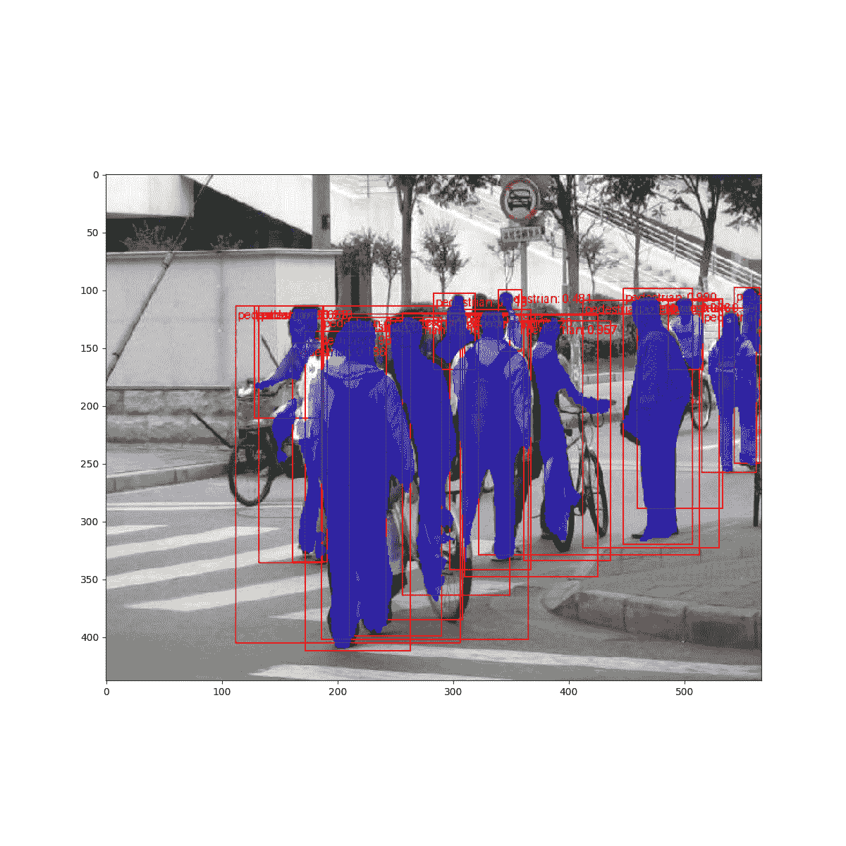
<matplotlib.image.AxesImage object at 0x7f48881f2830> 

结果看起来不错！

总结

在本教程中，您已经学会了如何为自定义数据集创建自己的目标检测模型训练流程。为此，您编写了一个torch.utils.data.Dataset类，该类返回图像和真实边界框以及分割掩模。您还利用了一个在 COCO train2017 上预训练的 Mask R-CNN 模型，以便在这个新数据集上进行迁移学习。

要查看包括多机器/多 GPU 训练在内的更完整示例，请查看 references/detection/train.py，该文件位于 torchvision 仓库中。

脚本的总运行时间：（2 分钟 27.747 秒）

下载 Python 源代码：torchvision_tutorial.py

下载 Jupyter 笔记本：torchvision_tutorial.ipynb

Sphinx-Gallery 生成的画廊

计算机视觉迁移学习教程

原文：pytorch.org/tutorials/beginner/transfer_learning_tutorial.html

译者：飞龙

协议：CC BY-NC-SA 4.0

注意

点击这里下载完整的示例代码

作者：Sasank Chilamkurthy

在本教程中，您将学习如何使用迁移学习训练卷积神经网络进行图像分类。您可以在cs231n 笔记中关于迁移学习的信息

引用这些笔记，

实际上，很少有人从头开始训练整个卷积网络（使用随机初始化），因为拥有足够大小的数据集相对较少。相反，通常是在非常大的数据集上预训练一个卷积网络（例如 ImageNet，其中包含 120 万张带有 1000 个类别的图像），然后将卷积网络用作感兴趣任务的初始化或固定特征提取器。

这两种主要的迁移学习场景如下：

• 微调卷积网络：与随机初始化不同，我们使用预训练网络来初始化网络，比如在 imagenet 1000 数据集上训练的网络。其余的训练看起来和往常一样。

• 卷积网络作为固定特征提取器：在这里，我们将冻结所有网络的权重，除了最后的全连接层之外。这个最后的全连接层被替换为一个具有随机权重的新层，只训练这一层。

# License: BSD
# Author: Sasank Chilamkurthyimport torch
import torch.nn as nn
import torch.optim as optim
from torch.optim import lr_scheduler
import torch.backends.cudnn as cudnn
import numpy as np
import torchvision
from torchvision import datasets, models, transforms
import matplotlib.pyplot as plt
import time
import os
from PIL import Image
from tempfile import TemporaryDirectorycudnn.benchmark = True
plt.ion()   # interactive mode 

<contextlib.ExitStack object at 0x7f6aede85450> 

加载数据

我们将使用 torchvision 和 torch.utils.data 包来加载数据。

我们今天要解决的问题是训练一个模型来分类蚂蚁和蜜蜂。我们每类有大约 120 张蚂蚁和蜜蜂的训练图像。每个类别有 75 张验证图像。通常，如果从头开始训练，这是一个非常小的数据集来进行泛化。由于我们使用迁移学习，我们应该能够相当好地泛化。

这个数据集是 imagenet 的一个非常小的子集。

注意

从这里下载数据并将其解压到当前目录。

# Data augmentation and normalization for training
# Just normalization for validation
data_transforms = {'train': transforms.Compose([transforms.RandomResizedCrop(224),transforms.RandomHorizontalFlip(),transforms.ToTensor(),transforms.Normalize([0.485, 0.456, 0.406], [0.229, 0.224, 0.225])]),'val': transforms.Compose([transforms.Resize(256),transforms.CenterCrop(224),transforms.ToTensor(),transforms.Normalize([0.485, 0.456, 0.406], [0.229, 0.224, 0.225])]),
}data_dir = 'data/hymenoptera_data'
image_datasets = {x: datasets.ImageFolder(os.path.join(data_dir, x),data_transforms[x])for x in ['train', 'val']}
dataloaders = {x: torch.utils.data.DataLoader(image_datasets[x], batch_size=4,shuffle=True, num_workers=4)for x in ['train', 'val']}
dataset_sizes = {x: len(image_datasets[x]) for x in ['train', 'val']}
class_names = image_datasets['train'].classesdevice = torch.device("cuda:0" if torch.cuda.is_available() else "cpu") 

可视化一些图像

让我们可视化一些训练图像，以便了解数据增强。

def imshow(inp, title=None):"""Display image for Tensor."""inp = inp.numpy().transpose((1, 2, 0))mean = np.array([0.485, 0.456, 0.406])std = np.array([0.229, 0.224, 0.225])inp = std * inp + meaninp = np.clip(inp, 0, 1)plt.imshow(inp)if title is not None:plt.title(title)plt.pause(0.001)  # pause a bit so that plots are updated# Get a batch of training data
inputs, classes = next(iter(dataloaders['train']))# Make a grid from batch
out = torchvision.utils.make_grid(inputs)imshow(out, title=[class_names[x] for x in classes]) 

![[‘蚂蚁’，‘蚂蚁’，‘蚂蚁’，‘蚂蚁’]]（…/Images/be538c850b645a41a7a77ff388954e14.png）

训练模型

现在，让我们编写一个通用的函数来训练一个模型。在这里，我们将说明：

• 调整学习率

• 保存最佳模型

在下面，参数scheduler是来自torch.optim.lr_scheduler的 LR 调度器对象。

def train_model(model, criterion, optimizer, scheduler, num_epochs=25):since = time.time()# Create a temporary directory to save training checkpointswith TemporaryDirectory() as tempdir:best_model_params_path = os.path.join(tempdir, 'best_model_params.pt')torch.save(model.state_dict(), best_model_params_path)best_acc = 0.0for epoch in range(num_epochs):print(f'Epoch {epoch}/{num_epochs  -  1}')print('-' * 10)# Each epoch has a training and validation phasefor phase in ['train', 'val']:if phase == 'train':model.train()  # Set model to training modeelse:model.eval()   # Set model to evaluate moderunning_loss = 0.0running_corrects = 0# Iterate over data.for inputs, labels in dataloaders[phase]:inputs = inputs.to(device)labels = labels.to(device)# zero the parameter gradientsoptimizer.zero_grad()# forward# track history if only in trainwith torch.set_grad_enabled(phase == 'train'):outputs = model(inputs)_, preds = torch.max(outputs, 1)loss = criterion(outputs, labels)# backward + optimize only if in training phaseif phase == 'train':loss.backward()optimizer.step()# statisticsrunning_loss += loss.item() * inputs.size(0)running_corrects += torch.sum(preds == labels.data)if phase == 'train':scheduler.step()epoch_loss = running_loss / dataset_sizes[phase]epoch_acc = running_corrects.double() / dataset_sizes[phase]print(f'{phase} Loss: {epoch_loss:.4f} Acc: {epoch_acc:.4f}')# deep copy the modelif phase == 'val' and epoch_acc > best_acc:best_acc = epoch_acctorch.save(model.state_dict(), best_model_params_path)print()time_elapsed = time.time() - sinceprint(f'Training complete in {time_elapsed  //  60:.0f}m {time_elapsed  %  60:.0f}s')print(f'Best val Acc: {best_acc:4f}')# load best model weightsmodel.load_state_dict(torch.load(best_model_params_path))return model 

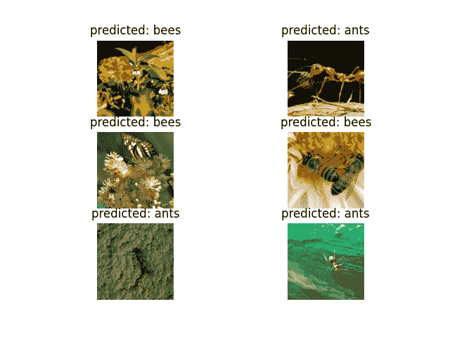
可视化模型预测

用于显示几张图像预测的通用函数

def visualize_model(model, num_images=6):was_training = model.trainingmodel.eval()images_so_far = 0fig = plt.figure()with torch.no_grad():for i, (inputs, labels) in enumerate(dataloaders['val']):inputs = inputs.to(device)labels = labels.to(device)outputs = model(inputs)_, preds = torch.max(outputs, 1)for j in range(inputs.size()[0]):images_so_far += 1ax = plt.subplot(num_images//2, 2, images_so_far)ax.axis('off')ax.set_title(f'predicted: {class_names[preds[j]]}')imshow(inputs.cpu().data[j])if images_so_far == num_images:model.train(mode=was_training)returnmodel.train(mode=was_training) 

微调卷积网络

加载一个预训练模型并重置最终的全连接层。

model_ft = models.resnet18(weights='IMAGENET1K_V1')
num_ftrs = model_ft.fc.in_features
# Here the size of each output sample is set to 2.
# Alternatively, it can be generalized to ``nn.Linear(num_ftrs, len(class_names))``.
model_ft.fc = nn.Linear(num_ftrs, 2)model_ft = model_ft.to(device)criterion = nn.CrossEntropyLoss()# Observe that all parameters are being optimized
optimizer_ft = optim.SGD(model_ft.parameters(), lr=0.001, momentum=0.9)# Decay LR by a factor of 0.1 every 7 epochs
exp_lr_scheduler = lr_scheduler.StepLR(optimizer_ft, step_size=7, gamma=0.1) 

Downloading: "https://download.pytorch.org/models/resnet18-f37072fd.pth" to /var/lib/jenkins/.cache/torch/hub/checkpoints/resnet18-f37072fd.pth0%|          | 0.00/44.7M [00:00<?, ?B/s]31%|###       | 13.7M/44.7M [00:00<00:00, 143MB/s]62%|######2   | 27.8M/44.7M [00:00<00:00, 146MB/s]94%|#########3| 41.9M/44.7M [00:00<00:00, 147MB/s]
100%|##########| 44.7M/44.7M [00:00<00:00, 146MB/s] 

训练和评估

在 CPU 上应该需要大约 15-25 分钟。但在 GPU 上，不到一分钟。

model_ft = train_model(model_ft, criterion, optimizer_ft, exp_lr_scheduler,num_epochs=25) 

Epoch 0/24
----------
train Loss: 0.4785 Acc: 0.7582
val Loss: 0.2864 Acc: 0.8758Epoch 1/24
----------
train Loss: 0.5262 Acc: 0.8074
val Loss: 0.5643 Acc: 0.7778Epoch 2/24
----------
train Loss: 0.4336 Acc: 0.8156
val Loss: 0.2852 Acc: 0.9020Epoch 3/24
----------
train Loss: 0.6358 Acc: 0.7582
val Loss: 0.4226 Acc: 0.8627Epoch 4/24
----------
train Loss: 0.4319 Acc: 0.8525
val Loss: 0.3289 Acc: 0.8824Epoch 5/24
----------
train Loss: 0.4856 Acc: 0.7869
val Loss: 0.3162 Acc: 0.8758Epoch 6/24
----------
train Loss: 0.3984 Acc: 0.8197
val Loss: 0.4864 Acc: 0.8235Epoch 7/24
----------
train Loss: 0.3621 Acc: 0.8238
val Loss: 0.2516 Acc: 0.8889Epoch 8/24
----------
train Loss: 0.2331 Acc: 0.9016
val Loss: 0.2395 Acc: 0.9085Epoch 9/24
----------
train Loss: 0.2571 Acc: 0.9016
val Loss: 0.2579 Acc: 0.9281Epoch 10/24
----------
train Loss: 0.3528 Acc: 0.8320
val Loss: 0.2281 Acc: 0.9150Epoch 11/24
----------
train Loss: 0.3108 Acc: 0.8320
val Loss: 0.2832 Acc: 0.9020Epoch 12/24
----------
train Loss: 0.2189 Acc: 0.8975
val Loss: 0.2734 Acc: 0.8824Epoch 13/24
----------
train Loss: 0.2872 Acc: 0.8648
val Loss: 0.2274 Acc: 0.9281Epoch 14/24
----------
train Loss: 0.2745 Acc: 0.8689
val Loss: 0.2712 Acc: 0.8954Epoch 15/24
----------
train Loss: 0.3152 Acc: 0.8689
val Loss: 0.3225 Acc: 0.8954Epoch 16/24
----------
train Loss: 0.2069 Acc: 0.9016
val Loss: 0.2486 Acc: 0.9085Epoch 17/24
----------
train Loss: 0.2447 Acc: 0.9016
val Loss: 0.2282 Acc: 0.9281Epoch 18/24
----------
train Loss: 0.2709 Acc: 0.8811
val Loss: 0.2590 Acc: 0.9020Epoch 19/24
----------
train Loss: 0.1959 Acc: 0.9139
val Loss: 0.2282 Acc: 0.9150Epoch 20/24
----------
train Loss: 0.2432 Acc: 0.8852
val Loss: 0.2623 Acc: 0.9150Epoch 21/24
----------
train Loss: 0.2643 Acc: 0.8770
val Loss: 0.2776 Acc: 0.9150Epoch 22/24
----------
train Loss: 0.2973 Acc: 0.8770
val Loss: 0.2362 Acc: 0.9020Epoch 23/24
----------
train Loss: 0.2859 Acc: 0.8648
val Loss: 0.2551 Acc: 0.9085Epoch 24/24
----------
train Loss: 0.3264 Acc: 0.8811
val Loss: 0.2317 Acc: 0.9150Training complete in 1m 3s
Best val Acc: 0.928105 

visualize_model(model_ft) 

卷积网络作为固定特征提取器

在这里，我们需要冻结除最后一层之外的所有网络。我们需要将requires_grad = False设置为冻结参数，以便在backward()中不计算梯度。

您可以在文档中信息这里。

model_conv = torchvision.models.resnet18(weights='IMAGENET1K_V1')
for param in model_conv.parameters():param.requires_grad = False# Parameters of newly constructed modules have requires_grad=True by default
num_ftrs = model_conv.fc.in_features
model_conv.fc = nn.Linear(num_ftrs, 2)model_conv = model_conv.to(device)criterion = nn.CrossEntropyLoss()# Observe that only parameters of final layer are being optimized as
# opposed to before.
optimizer_conv = optim.SGD(model_conv.fc.parameters(), lr=0.001, momentum=0.9)# Decay LR by a factor of 0.1 every 7 epochs
exp_lr_scheduler = lr_scheduler.StepLR(optimizer_conv, step_size=7, gamma=0.1) 

训练和评估

在 CPU 上，这将比以前的情况快大约一半的时间。这是预期的，因为大部分网络不需要计算梯度。然而，前向计算是需要的。

model_conv = train_model(model_conv, criterion, optimizer_conv,exp_lr_scheduler, num_epochs=25) 

Epoch 0/24
----------
train Loss: 0.6996 Acc: 0.6516
val Loss: 0.2014 Acc: 0.9346Epoch 1/24
----------
train Loss: 0.4233 Acc: 0.8033
val Loss: 0.2656 Acc: 0.8758Epoch 2/24
----------
train Loss: 0.4603 Acc: 0.7869
val Loss: 0.1847 Acc: 0.9477Epoch 3/24
----------
train Loss: 0.3096 Acc: 0.8566
val Loss: 0.1747 Acc: 0.9477Epoch 4/24
----------
train Loss: 0.4427 Acc: 0.8156
val Loss: 0.1630 Acc: 0.9477Epoch 5/24
----------
train Loss: 0.5505 Acc: 0.7828
val Loss: 0.1643 Acc: 0.9477Epoch 6/24
----------
train Loss: 0.3004 Acc: 0.8607
val Loss: 0.1744 Acc: 0.9542Epoch 7/24
----------
train Loss: 0.4083 Acc: 0.8361
val Loss: 0.1892 Acc: 0.9412Epoch 8/24
----------
train Loss: 0.4483 Acc: 0.7910
val Loss: 0.1984 Acc: 0.9477Epoch 9/24
----------
train Loss: 0.3335 Acc: 0.8279
val Loss: 0.1942 Acc: 0.9412Epoch 10/24
----------
train Loss: 0.2413 Acc: 0.8934
val Loss: 0.2001 Acc: 0.9477Epoch 11/24
----------
train Loss: 0.3107 Acc: 0.8689
val Loss: 0.1801 Acc: 0.9412Epoch 12/24
----------
train Loss: 0.3032 Acc: 0.8689
val Loss: 0.1669 Acc: 0.9477Epoch 13/24
----------
train Loss: 0.3587 Acc: 0.8525
val Loss: 0.1900 Acc: 0.9477Epoch 14/24
----------
train Loss: 0.2771 Acc: 0.8893
val Loss: 0.2317 Acc: 0.9216Epoch 15/24
----------
train Loss: 0.3064 Acc: 0.8852
val Loss: 0.1909 Acc: 0.9477Epoch 16/24
----------
train Loss: 0.4243 Acc: 0.8238
val Loss: 0.2227 Acc: 0.9346Epoch 17/24
----------
train Loss: 0.3297 Acc: 0.8238
val Loss: 0.1916 Acc: 0.9412Epoch 18/24
----------
train Loss: 0.4235 Acc: 0.8238
val Loss: 0.1766 Acc: 0.9477Epoch 19/24
----------
train Loss: 0.2500 Acc: 0.8934
val Loss: 0.2003 Acc: 0.9477Epoch 20/24
----------
train Loss: 0.2413 Acc: 0.8934
val Loss: 0.1821 Acc: 0.9477Epoch 21/24
----------
train Loss: 0.3762 Acc: 0.8115
val Loss: 0.1842 Acc: 0.9412Epoch 22/24
----------
train Loss: 0.3485 Acc: 0.8566
val Loss: 0.2166 Acc: 0.9281Epoch 23/24
----------
train Loss: 0.3625 Acc: 0.8361
val Loss: 0.1747 Acc: 0.9412Epoch 24/24
----------
train Loss: 0.3840 Acc: 0.8320
val Loss: 0.1768 Acc: 0.9412Training complete in 0m 31s
Best val Acc: 0.954248 

visualize_model(model_conv)plt.ioff()
plt.show() 

对自定义图像进行推断

使用训练好的模型对自定义图像进行预测并可视化预测的类标签以及图像。

def visualize_model_predictions(model,img_path):was_training = model.trainingmodel.eval()img = Image.open(img_path)img = data_transforms'val'img = img.unsqueeze(0)img = img.to(device)with torch.no_grad():outputs = model(img)_, preds = torch.max(outputs, 1)ax = plt.subplot(2,2,1)ax.axis('off')ax.set_title(f'Predicted: {class_names[preds[0]]}')imshow(img.cpu().data[0])model.train(mode=was_training) 

visualize_model_predictions(model_conv,img_path='data/hymenoptera_data/val/bees/72100438_73de9f17af.jpg'
)plt.ioff()
plt.show() 

进一步学习

如果您想了解更多关于迁移学习应用的信息，请查看我们的计算机视觉迁移学习量化教程。

脚本的总运行时间：（1 分钟 36.689 秒）

下载 Python 源代码：transfer_learning_tutorial.py

下载 Jupyter 笔记本：transfer_learning_tutorial.ipynb

Sphinx-Gallery 生成的图库