数据挖掘与分析部分实验与实训项目报告

一、机器学习算法的应用

1. 朴素贝叶斯分类器

相关代码

import pandas as pd
from sklearn.model_selection import train_test_split
from sklearn.naive_bayes import GaussianNB, MultinomialNB
from sklearn.metrics import accuracy_score
# 将数据加载到DataFrame中，删除ID和ZIP Code列
df = pd.read_csv('universalbank.csv')
df = df.drop(columns=['ID', 'ZIP Code'])
# 以下是使用高斯朴素贝叶斯分类器的代码
# 分离特征和目标变量
X = df.drop(columns=['Personal Loan'])
y = df['Personal Loan']
# 划分数据集
# X_train, X_test, y_train, y_test = train_test_split(X, y, test_size=0.3, random_state=42)
X_train, X_test, y_train, y_test = train_test_split(X, y, test_size=0.3, random_state=0)
# 创建高斯朴素贝叶斯分类器实例
gnb = GaussianNB()
# 训练模型
gnb.fit(X_train, y_train)
# 预测测试集
y_pred = gnb.predict(X_test)
# 输出预测结果和模型准确度
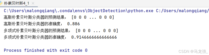
print("高斯朴素贝叶斯分类器的预测结果：", y_pred)
print("高斯朴素贝叶斯分类器的准确度：", accuracy_score(y_test, y_pred))
# 以下是使用多项式朴素贝叶斯分类器的代码
# 筛选出离散型特征
X_discrete = df[['Family', 'Education', 'Securities Account', 'CD Account', 'Online', 'CreditCard']]
# 划分数据集
# X_train_discrete, X_test_discrete, y_train, y_test = train_test_split(X_discrete, y, test_size=0.3, random_state=42)
X_train_discrete, X_test_discrete, y_train, y_test = train_test_split(X_discrete, y, test_size=0.3, random_state=0)
# 创建多项式朴素贝叶斯分类器实例
mnb = MultinomialNB()
# 训练模型
mnb.fit(X_train_discrete, y_train)
# 预测测试集
y_pred_discrete = mnb.predict(X_test_discrete)
# 输出预测结果和模型准确度
print("多项式朴素贝叶斯分类器的预测结果：", y_pred_discrete)
print("多项式朴素贝叶斯分类器的准确度：", accuracy_score(y_test, y_pred_discrete))

运行结果

2.K近邻分类器（KNN）

相关代码

import pandas as pd
from sklearn.model_selection import train_test_split
from sklearn.neighbors import KNeighborsClassifier
from sklearn.metrics import accuracy_score# 将数据加载到DataFrame中，删除ID和ZIP Code列
df = pd.read_csv('universalbank.csv')
df = df.drop(columns=['ID', 'ZIP Code'])
# 分离特征和目标变量
X = df.drop(columns=['Personal Loan'])
y = df['Personal Loan']
# 划分数据集
X_train, X_test, y_train, y_test = train_test_split(X, y, test_size=0.3, random_state=0)
# 创建KNN分类器实例，设置最近邻的数量K为5
knn = KNeighborsClassifier(n_neighbors=5)
# 训练模型
knn.fit(X_train, y_train)
# 预测测试集
y_pred = knn.predict(X_test)
# 输出预测结果和模型准确度
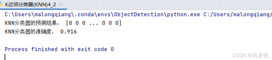
print("KNN分类器的预测结果：", y_pred)
print("KNN分类器的准确度：", accuracy_score(y_test, y_pred))

运行结果

3. CART决策树

相关代码

import pandas as pd
from sklearn.model_selection import train_test_split
from sklearn.tree import DecisionTreeClassifier
from sklearn.metrics import accuracy_score
from sklearn.tree import export_graphviz
import graphviz
# 将数据加载到DataFrame中，删除ID和ZIP Code列
df = pd.read_csv('universalbank.csv')
df = df.drop(columns=['ID', 'ZIP Code'])
# 分离特征和目标变量
X = df.drop(columns=['Personal Loan'])
y = df['Personal Loan']
# 划分数据集
X_train, X_test, y_train, y_test = train_test_split(X, y, test_size=0.3, random_state=0)
# 创建CART决策树分类器实例，设置决策树的深度限制为10层
dt = DecisionTreeClassifier(max_depth=10, random_state=42)
# 训练模型
dt.fit(X_train, y_train)
# 预测测试集
y_pred = dt.predict(X_test)
# 输出预测结果和模型准确度
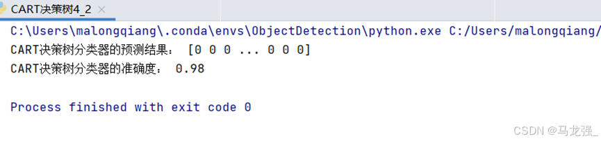
print("CART决策树分类器的预测结果：", y_pred)
print("CART决策树分类器的准确度：", accuracy_score(y_test, y_pred))# 可视化训练好的CART决策树模型
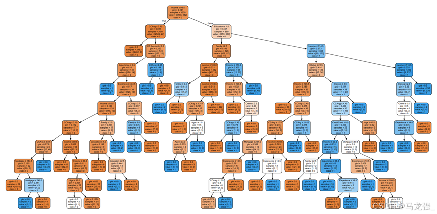
dot_data = export_graphviz(dt, out_file=None,feature_names=X.columns,class_names=['0', '1'],filled=True, rounded=True,special_characters=True)
graph = graphviz.Source(dot_data)
graph.render("universalbank_decision_tree")  # 保存为PDF文件
graph.view()  # 在默认PDF查看器中打开

运行结果

4.神经网络回归任务

相关代码

import pandas as pd
import numpy as np
from sklearn.model_selection import train_test_split
from sklearn.neural_network import MLPRegressordata = pd.read_csv('house-price.csv')
X = data.iloc[:, 2:14]
y = data.iloc[:, [1]]# 划分数据集，70%为训练集，30%为测试集
X_train, X_test, y_train, y_test = train_test_split(X, y, test_size=0.3, random_state=0)# 创建多层感知机回归模型实例，设置隐藏层层数和神经元数量
regressor = MLPRegressor(hidden_layer_sizes=(100, 10), activation="relu")# 使用训练集数据训练模型
regressor.fit(X_train, y_train)# 使用训练好的模型对测试集进行预测
y_pred = regressor.predict(X_test)# 计算模型的均方误差（MSE）
mse = np.sum(np.square(y_pred - y_test.values)) / len(y_test)
# 计算模型的平均绝对误差（MAE）
mae = np.sum(np.abs(y_pred - y_test.values)) / len(y_test)# 输出测试数据的预测结果和模型的MSE和MAE
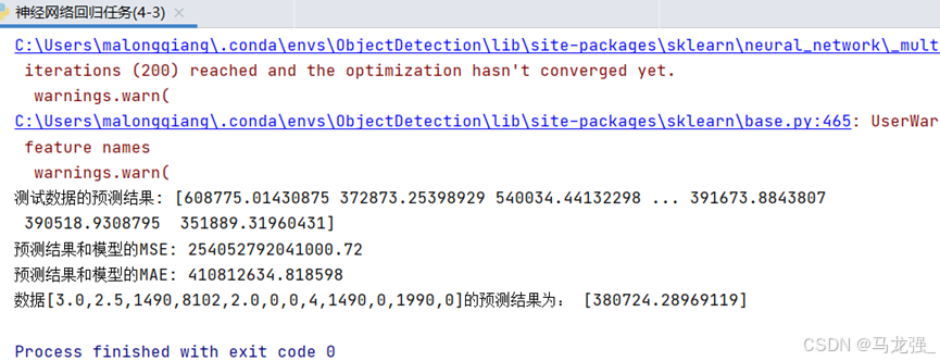
print('测试数据的预测结果:', y_pred)
print("预测结果和模型的MSE:", mse)
print("预测结果和模型的MAE:", mae)
# 使用训练好的模型对给定的数据进行房价预测
y_ = regressor.predict(np.array([[3.0, 2.5, 1490, 8102, 2.0, 0, 0, 4, 1490, 0, 1990, 0]]))
print('数据[3.0,2.5,1490,8102,2.0,0,0,4,1490,0,1990,0]的预测结果为：', y_)

运行结果

5.神经网络分类任务

相关代码

import pandas as pd
from sklearn.neural_network import MLPClassifier
from sklearn.metrics import accuracy_score# 将数据加载到DataFrame中
df = pd.read_excel('企业贷款审批数据表.xlsx')
# 选择特征列和目标列
X = df.iloc[:, 1:4]  # 特征列X1, X2, X3
y = df.iloc[:, 4]    # 目标列Y
# 使用前10行数据作为训练集，11-20行数据作为测试集
X_train = X.iloc[:10]
y_train = y.iloc[:10]
X_test = X.iloc[10:20]
y_test = y.iloc[10:20]
# 创建MLP分类模型实例，设置隐藏层层数和神经元数量
mlp = MLPClassifier(hidden_layer_sizes=(10,5), max_iter=1000, random_state=0,verbose=1)
# 训练模型
mlp.fit(X_train, y_train)
# 使用训练好的模型对测试集进行预测
y_pred = mlp.predict(X_test)
# 计算模型的准确度
accuracy = accuracy_score(y_test, y_pred)
# 输出预测结果和模型准确度
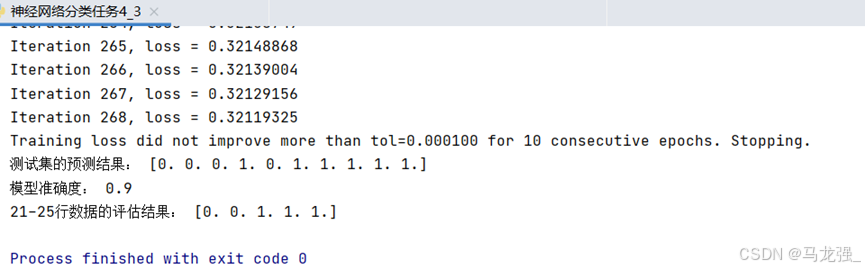
print("测试集的预测结果：", y_pred)
print("模型准确度：", accuracy)
# 使用训练好的模型对21-25行数据进行预测
# 给定的数据
new_data = df.iloc[20:, 1:4]
predicted_results = mlp.predict(new_data)
# 输出评估结果
print("21-25行数据的评估结果：", predicted_results)

运行结果

6. 关联规则分析

相关代码

import pandas as pd
from mlxtend.preprocessing import TransactionEncoder
from tabulate import tabulate
from mlxtend.frequent_patterns import apriori, fpgrowth, association_rules# （2）数据读取与预处理
data = pd.read_excel('tr.xlsx', keep_default_na=False)
# 将数据转换为适合TransactionEncoder的格式
te = TransactionEncoder()
te_ary = te.fit(data.values).transform(data.values)
# 创建DataFrame
df = pd.DataFrame(te_ary, columns=te.columns_)
# 剔除第3列到第6列
df = df.drop(columns=df.columns[0:9])
# 将True和False替换为1和0
df = df.replace({True: 1, False: 0})
# 使用tabulate库打印DataFrame
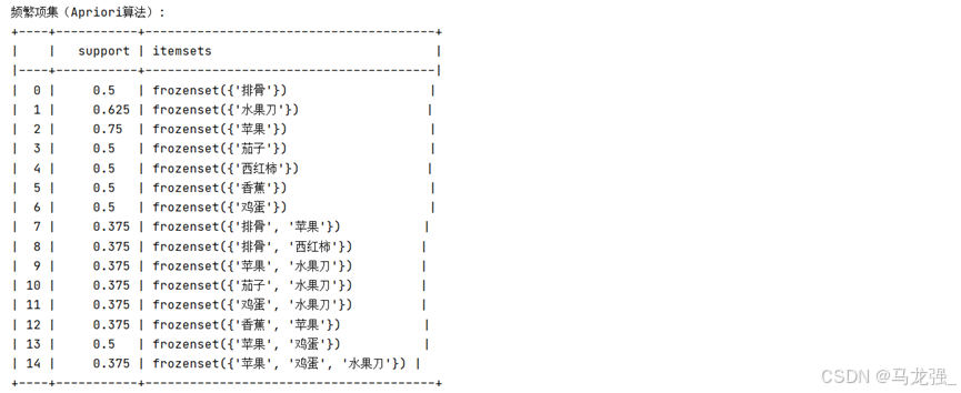
# print(tabulate(df, headers='keys', tablefmt='psql'))# （3）使用apriori算法挖掘频繁项集（最小支持度为0.3）
frequent_itemsets_apriori = apriori(df, min_support=0.3, use_colnames=True)# （4）使用FP-growth算法挖掘频繁项集（最小支持度为0.3）
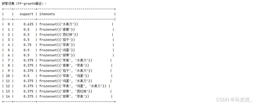
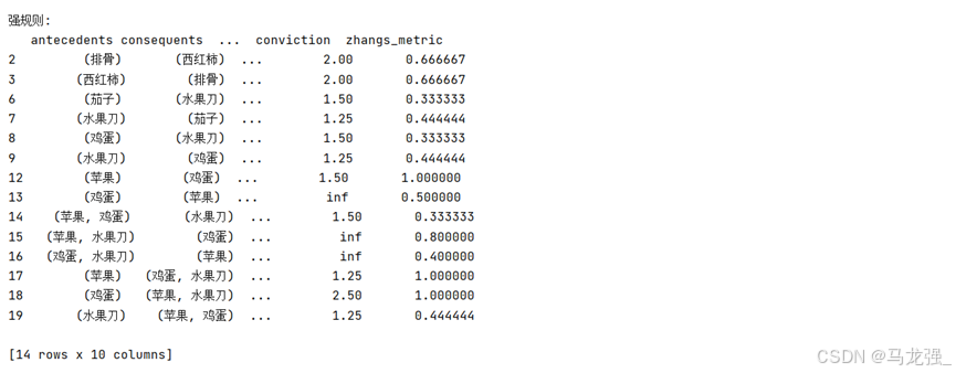
frequent_itemsets_fpgrowth = fpgrowth(df, min_support=0.3, use_colnames=True)# （5）生成强规则(最小置信度为0.5, 提升度>1)
rules = association_rules(frequent_itemsets_apriori, metric='confidence', min_threshold=0.5, support_only=False)
rules = rules[rules['lift'] > 1]# 输出结果
print("频繁项集（Apriori算法）:")
# print(frequent_itemsets_apriori)
print(tabulate(frequent_itemsets_apriori, headers='keys', tablefmt='psql'))
print("\n频繁项集（FP-growth算法）:")
# print(frequent_itemsets_fpgrowth)
print(tabulate(frequent_itemsets_fpgrowth, headers='keys', tablefmt='psql'))
print("\n强规则:")
print(rules)

运行结果

7.时间序列分析

相关代码

import pandas as pd
import warnings
from matplotlib import MatplotlibDeprecationWarning
import matplotlib.pyplot as plt
from statsmodels.graphics.tsaplots import plot_acf, plot_pacf
from statsmodels.tsa.stattools import adfuller as ADF
from statsmodels.tsa.arima.model import ARIMA# 屏蔽所有FutureWarning类型的警告
warnings.filterwarnings("ignore", category=FutureWarning)
warnings.filterwarnings("ignore", category=UserWarning, module="statsmodels")
warnings.filterwarnings("ignore", category=MatplotlibDeprecationWarning)# 读取数据
data = pd.read_csv('shampoo.csv')# 假设数据框中日期列名为'Month'
data['Month'] = '2024-' + data['Month']# 如果需要转换为日期类型（可选）
data['Month'] = pd.to_datetime(data['Month'], format='%Y-%m-%d')
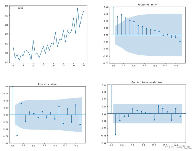
data.rename(columns={'Month': 'Date'}, inplace=True)# （3）检测序列的平稳性
# 时序图判断法
plt.rcParams['font.sans-serif'] = ['SimHei']
plt.rcParams['axes.unicode_minus'] = False
plt.plot(data['Sales'])
plt.legend(['Sales'])
plt.show()# 制自相关图判断法
plot_acf(data['Sales'])
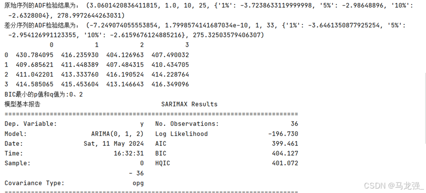
plt.show()# 使用ADF单位根检测法
print('原始序列的ADF检验结果为：', ADF(data['Sales']))# （4）差分处理
# 注意：根据上一步结果判断数据序列为非平稳序列，如想使用模型对数据进行建模，
# 则需将数据转换为平稳序列。所以在这一步使用差分处理对序列进行处理。
Date_data = data['Sales'].diff().dropna()# 对处理后的序列进行平稳性检测（自相关图法、偏相关图法、ADF检测法）
plot_acf(Date_data)
plt.show()
plot_pacf(Date_data)
plt.show()print('差分序列的ADF检验结果为：', ADF(Date_data))# （5）使用ARIMA模型对差分处理后的序列进行建模
# 选择合适的p和q值
pmax = int(len(Date_data)/10)
qmax = int(len(Date_data)/10)
bic_matrix = []
for p in range(pmax + 1):tmp = []for q in range(qmax + 1):try:tmp.append(ARIMA(data['Sales'].values, order=(p,1,q)).fit().bic)except:tmp.append(None)bic_matrix.append(tmp)
bic_matrix = pd.DataFrame(bic_matrix)p, q = bic_matrix.stack().idxmin()
print('BIC最小的p值和q值为:%s、%s' % (p, q))# 使用模型预测未来5个月的销售额
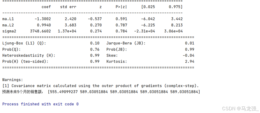
model = ARIMA(data['Sales'].values, order=(p,1,q)).fit()
print('模型基本报告', model.summary())
print('预测未来5个月的销售额：', model.forecast(5))

运行结果

二、深度学习算法应用

1. TensorFlow框架的基本使用

（1）获取训练数据

构建一个简单的线性模型：W，b为参数，W=2，b=1，运用tf.random.normal() 产生1000个随机数，产生x,y数据。

用matplotlib库，用蓝色绘制训练数据。

import tensorflow as tf
import numpy as np
import warnings
from matplotlib import MatplotlibDeprecationWarning# 屏蔽所有FutureWarning类型的警告
warnings.filterwarnings("ignore", category=FutureWarning)
warnings.filterwarnings("ignore", category=UserWarning, module="statsmodels")
warnings.filterwarnings("ignore", category=MatplotlibDeprecationWarning)
W = 3.0   # W参数设置
b =1.0    # b参数设置
num = 1000
# x随机输入
x = tf.random.normal(shape=[num])
# 随机偏差
c = tf.random.normal(shape=[num])
# 构造y数据
y = W * x + b + c
# print(x)# 画图观察
import matplotlib.pyplot as plt    #加载画图库
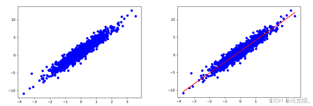
plt.scatter(x, y, c='b')    # 画离散图
plt.show()    # 展示图

（2）定义模型

通过对样本数据的离散图可以判断，呈线性规律变化，因此可以建立一个线性模型，即，把该线性模型定义为一个简单的类，里面封装了变量和计算，变量设置用tf.Variable()。

#定义模型
class LineModel(object):   # 定义一个LineModel的类def __init__(self):# 初始化变量self.W = tf.Variable(5.0)self.b = tf.Variable(0.0)def __call__(self, x):   #定义返回值return self.W * x + self.bdef train(self, x, y, learning_rate):   #定义训练函数with tf.GradientTape() as t:current_loss = loss(self.__call__(x), y)  #损失函数计算# 对W，b求导d_W, d_b = t.gradient(current_loss, [self.W, self.b])# 减去梯度*学习率self.W.assign_sub(d_W*learning_rate)  #减法操作self.b.assign_sub(d_b*learning_rate)

（3）定义损失函数

损失函数是衡量给定输入的模型输出与期望输出的匹配程度，采用均方误差（L2范数损失函数）。

# 定义损失函数
def loss(predicted_y, true_y):   # 定义损失函数return tf.reduce_mean(tf.square(true_y - predicted_y))  # 返回均方误差值

（4）模型训练

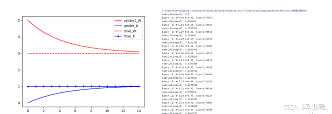
运用数据和模型来训练得到模型的变量（W和b），观察W和b的变化（使用matplotlib绘制W和b的变化情况曲线）。

# 求解过程     
model= LineModel()  #运用模型实例化
# 计算W，b参数值的变化
W_s, b_s = [], []    #增加新中间变量
for epoch in range(15):    #循环15次W_s.append(model.W.numpy())  #提取模型的W参数添加到中间变量w_sb_s.append(model.b.numpy())print('model.W.numpy():',model.W.numpy())# 计算损失函数losscurrent_loss = loss(model(x), y)model.train(x, y, learning_rate=0.1)   # 运用定义的train函数训练print('Epoch %2d: W=%1.2f b=%1.2f, loss=%2.5f' %(epoch, W_s[-1], b_s[-1], current_loss))    #输出训练情况
# 画图，把W,b的参数变化情况画出来
epochs = range(15)   #这个迭代数据与上面循环数据一样
plt.figure(1)
plt.scatter(x, y, c='b')    # 画离散图
plt.plot(x,model(x),c='r')
plt.figure(2)
plt.plot(epochs, W_s, 'r',epochs, b_s, 'b')  #画图
plt.plot([W] * len(epochs), 'r--',[b] * len(epochs), 'b-*')
plt.legend(['pridect_W', 'pridet_b', 'true_W', 'true_b'])  # 图例
plt.show()

运行结果

2. 多层神经网络分类

（1）数据获取与预处理

MNIST 数据集来自美国国家标准与技术研究所, National Institute of Standards and Technology (NIST). 训练集 (training set) 由来自 250 个不同人手写的数字构成, 其中 50% 是高中学生, 50% 来自人口普查局 (the Census Bureau) 的工作人员. 测试集(test set) 也是同样比例的手写数字数据。

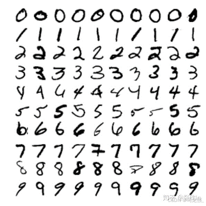
每张图像的大小都是28x28像素。MNIST数据集有60000张图像用于训练和10000张图像用于测试，其中每张图像都被标记了对应的数字（0-9）。

（2）加载数据集

import tensorflow as tf
import matplotlib.pyplot as plt
# 1. 数据获取与预处理
# 加载数据集
mnist = tf.keras.datasets.mnist
(x_train_all, y_train_all), (x_test, y_test) = mnist.load_data()

（3）查看数据集

def show_single_image(img_arr):plt.imshow(img_arr, cmap='binary')plt.show()show_single_image(x_train_all[0])

（4）归一化处理

x_train_all, x_test = x_train_all / 255.0, x_test / 255.0

模型构建

（5）模型定义

# 模型定义
model = tf.keras.models.Sequential([  #输入层  tf.keras.layers.Flatten(input_shape=(28, 28)),  #隐藏层1  tf.keras.layers.Dense(256, activation=tf.nn.relu),  #百分之20的神经元不工作，防止过拟合  tf.keras.layers.Dropout(0.2),  #隐藏层2  tf.keras.layers.Dense(128, activation=tf.nn.relu),  #隐藏层3  tf.keras.layers.Dense(64, activation=tf.nn.relu),  #输出层  tf.keras.layers.Dense(10, activation=tf.nn.softmax)  
])

（6）编译模型

#定义优化器，损失函数，训练效果中计算准确率  
model.compile(optimizer='adam', loss='sparse_categorical_crossentropy', metrics=['sparse_categorical_accuracy'])

（7）输出模型参数

# 打印网络参数
print(model.summary())

模型训练

（8）训练

# 训练模型
history = model.fit(x_train_all, y_train_all, epochs=50, validation_split=0.2, verbose=1)

（9）获取训练历史数据中的各指标值

acc = history.history['sparse_categorical_accuracy']
val_acc = history.history['val_sparse_categorical_accuracy']
loss = history.history['loss']
val_loss = history.history['val_loss']

（10）绘制指标在训练过程中的变化图

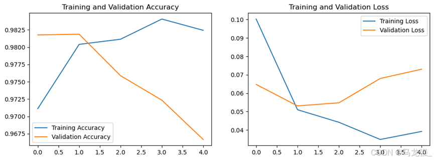
plt.figure(1)
plt.plot(acc, label='Training Accuracy')
plt.plot(val_acc, label='Validation Accuracy')
plt.title('Training and Validation Accuracy')
plt.legend()
plt.figure(2)
plt.plot(loss, label='Training Loss')
plt.plot(val_loss, label='Validation Loss')
plt.title('Training and Validation Loss')
plt.legend()
plt.show()

（11）模型评估

使用测试集对模型进行评估

loss, accuracy = model.evaluate(x_test, y_test, verbose=1)
print(f"Test Loss: {loss}, Test Accuracy: {accuracy}")

3. 多层神经网络回归

（1）数据获取与预处理

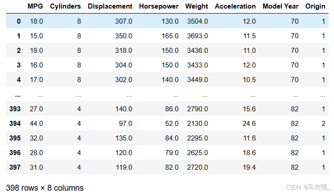
Auto MPG 数据集，它记录了各种汽车效能指标MPG(Mile Per Gallon)与气缸数、重量、马力等因素的真实数据。除了产地的数字字段表示类别外，其他字段都是数值类型。对于产地地段，1 表示美国，2 表示欧洲，3 表示日本。

（2）加载数据集

import pandas as pd
import numpy as np
import seaborn as sns
import matplotlib.pyplot as plt
from sklearn.preprocessing import StandardScaler
from sklearn.model_selection import train_test_split
from tensorflow.keras.models import Sequential
from tensorflow.keras.layers import Dense
column_names = ['MPG', 'Cylinders', 'Displacement', 'Horsepower', 'Weight','Acceleration', 'Model Year', 'Origin']
raw_dataset = pd.read_csv('./data/auto-mpg.data', names=column_names,na_values="?", comment='\t',sep=" ", skipinitialspace=True)

（3）数据清洗

# 数据清洗
# 统计每列的空值数量
null_counts = raw_dataset.isnull().sum()
# 打印每列的空值数量
print(null_counts)
# 删除包含空值的行
dataset = raw_dataset.dropna()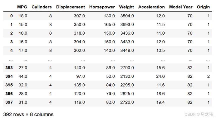

（4）将Origin列转换为one-hot（独热）编码。

dataset = pd.get_dummies(dataset, columns=['Origin'])

（5）数据探索

使用describe方法查看数据的统计指标

# 使用describe方法查看数据的统计指标
dataset.describe()

使用seaborn库中pairplot方法绘制"MPG", "Cylinders", "Displacement", "Weight"四列的联合分布图

# 使用seaborn库中pairplot方法绘制"MPG", "Cylinders", "Displacement", "Weight"四列的联合分布图
sns.pairplot(dataset[['MPG', 'Cylinders', 'Displacement', 'Weight']])

（6）数据可视化

labels = dataset.pop('MPG')  #从数据集中取出目标值MPG
#数据标准化
from sklearn.preprocessing import StandardScaler
def norm(x):return (x - train_stats['mean']) / train_stats['std'] #标准化公式
scaler = StandardScaler()
normed_dataset = scaler.fit_transform(dataset)

（7）划分数据集

X_train, X_test, Y_train, Y_test = train_test_split(normed_dataset, labels, test_size=0.2, random_state=0)

模型构建

（8）模型定义

import tensorflow as tf
model = tf.keras.Sequential([tf.keras.layers.Dense(64, activation='relu', input_shape=[X_train.shape[1]]),tf.keras.layers.Dense(64, activation='relu'),tf.keras.layers.Dense(1)])

（9）模型编译

model.compile(loss='mse', optimizer='adam', metrics=['mae', 'mse'])
plt.show()

（10）输出模型参数

# 输出模型参数
print(model.summary())

模型训练

（11）训练

history = model.fit(X_train, Y_train, epochs=100, validation_split=0.2, verbose=1)

（12）获取训练历史数据中的各指标值

mae = history.history['mae']
val_mae = history.history['val_mae']
mse = history.history['mse']
val_mse = history.history['val_mse']

（13）绘制指标在训练过程中的变化图

plt.figure(figsize=(12, 4))
plt.subplot(1, 2, 1)
plt.plot(mae, label='Training MAE')
plt.plot(val_mae, label='Validation MAE')
plt.title('Training and Validation MAE')
plt.legend()
plt.subplot(1, 2, 2)
plt.plot(mse, label='Training MSE')
plt.plot(val_mse, label='Validation MSE')
plt.title('Training and Validation MSE')
plt.legend()
plt.show()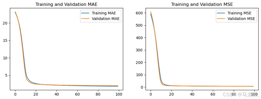

（14）模型评估

使用测试集对模型进行评估

model.evaluate(X_test, Y_test, verbose=1)

4. 多层神经网络回归

（1）数据获取与预处理

IMDB数据集，有5万条来自网络电影数据库的评论，其中25000千条用来训练，25000用来测试，每个部分正负评论各占50%。和MNIST数据集类似，IMDB数据集也集成在Keras中，同时经过了预处理：电影评论转换成了一系列数字，每个数字代表字典中的一个单词（表示该单词出现频率的排名）

（2）读取数据

from tensorflow.keras.datasets import imdb
from tensorflow.keras.preprocessing.sequence import pad_sequences
from tensorflow.keras.models import Sequential
from tensorflow.keras.layers import Embedding, LSTM, Dense
from tensorflow.keras.callbacks import EarlyStopping
import tensorflow as tf
# 加载数据,评论文本已转换为整数，其中每个整数表示字典中的特定单词
(x_train, y_train), (x_test, y_test) = imdb.load_data(num_words=10000)

（2）预处理

# 循环神经网络输入长度固定
# 这里应该注意，循环神经网络的输入是固定长度的，否则运行后会出错。
# 由于电影评论的长度必须相同，pad_sequences 函数来标准化评论长度
x_train = tf.keras.preprocessing.sequence.pad_sequences(x_train, maxlen=100)
x_test = tf.keras.preprocessing.sequence.pad_sequences(x_test, maxlen=100)

模型搭建

（3）模型定义

model = Sequential([#定义嵌入层Embedding(10000,  # 词汇表大小中收录单词数量，也就是嵌入层矩阵的行数128,           # 每个单词的维度，也就是嵌入层矩阵的列数input_length=100),# 定义LSTM隐藏层LSTM(128, dropout=0.2, recurrent_dropout=0.2),# 模型输出层Dense(1, activation='sigmoid')
])

（4）编译模型

model.compile(loss='binary_crossentropy',optimizer='adam',metrics=['accuracy'])

模型训练

（5）训练

history = model.fit(x_train, y_train, epochs=5, validation_split=0.2, verbose=1)

（6）获取训练历史数据中的各指标值

accuracy = history.history['accuracy']
val_accuracy = history.history['val_accuracy']
loss = history.history['loss']
val_loss = history.history['val_loss']

（7）绘制指标在训练过程中的变化图

# 绘制指标在训练过程中的变化图
import matplotlib.pyplot as plt# plt.figure(1)
plt.figure(figsize=(12, 4))
plt.subplot(1, 2, 1)
plt.plot(accuracy, label='Training Accuracy')
plt.plot(val_accuracy, label='Validation Accuracy')
plt.title('Training and Validation Accuracy')
plt.legend()# plt.figure(2)
plt.subplot(1, 2, 2)
plt.plot(loss, label='Training Loss')
plt.plot(val_loss, label='Validation Loss')
plt.title('Training and Validation Loss')
plt.legend()
plt.show()

（8）模型评估

使用测试集对模型进行评估

test_loss, test_acc = model.evaluate(x_test, y_test, verbose=1)
print(f"Test Accuracy: {test_acc}, Test Loss: {test_loss}")

三、数据挖掘综合应用

1.微博评论情感分析

（1）数据读取

新浪微博数据集（网上搜集、作者不详）来源于网上的GitHub社区，有微博10 万多条，都带有情感标注，正负向评论约各 5 万条，用来做情感分析的数据集。

import jieba
import pandas as pd
import re
from wordcloud import WordCloud
import matplotlib.pyplot as plt
from keras.models import Sequential
from keras.layers import Embedding, LSTM, Dense
#from keras.preprocessing.text import Tokenizer
from keras.utils import to_categorical
from sklearn.model_selection import train_test_split
from keras.callbacks import EarlyStoppingdata = pd.read_csv("E:/课程内容文件/大三下学期/数据挖掘与分析/课程实验/实验六/weibo_senti_100.csv")

数据预处理

（2）分词

data['data_cut'] = data['review'].apply(lambda x: jieba.lcut(x))

（3）去停用词

with open("E:/课程内容文件/大三下学期/数据挖掘与分析-王思霖/课程实验/实验六/stopword.txt", 'r', encoding='utf-8') as f:stop = f.readlines()
stop = [re.sub('\n', '', r) for r in stop]
data['data_after'] = data['data_cut'].apply(lambda x: [i for i in x if i not in stop and i != '\ufeff'])

（4）词云分析

num_words = [''.join(i) for i in data['data_after']]
num_words = ''.join(num_words)
num = pd.Series(jieba.lcut(num_words)).value_counts()
wc_pic = WordCloud(background_color='white', font_path=r'C:\Windows\Fonts\simhei.ttf').fit_words(num)
plt.figure(figsize=(10, 10))
plt.imshow(wc_pic)
plt.axis('off')
plt.show()

（5）词向量

# 构建词向量矩阵
w = []
for i in data['data_after']:w.extend(i)
# 计算词频
word_counts = pd.Series(w).value_counts()
# 创建DataFrame
num_data = pd.DataFrame(word_counts).reset_index()
# 重命名列
num_data.columns = ['word', 'count']
# 添加id列
num_data['id'] = num_data.index + 1# 创建单词到ID的映射字典
word_to_id_dict = num_data.set_index('word')['id'].to_dict()# 优化的转化成数字函数
def optimized_word2num(x):return [word_to_id_dict[i] for i in x if i in word_to_id_dict]# 应用优化后的函数
data['vec'] = data['data_after'].apply(optimized_word2num)

（6）划分数据集

import tensorflow as tf
# from keras.preprocessing.text import Tokenizer
from tensorflow.keras.preprocessing.sequence import pad_sequencesmaxlen = 128
vec_data = pad_sequences(data['vec'], maxlen=maxlen)
x_train, x_test, y_train, y_test = train_test_split(vec_data, data['label'], test_size=0.2, random_state=0)

模型搭建

（7）模型定义

model = Sequential([Embedding(len(num_data) + 1,  # 词汇表大小中收录单词数量，加1是因为要包括未知词64,  # 每个单词的维度input_length=maxlen),LSTM(64, dropout=0.2, recurrent_dropout=0.2),Dense(1, activation='sigmoid')
])

（8）编译模型

model.compile(loss='binary_crossentropy',optimizer='adam',metrics=['accuracy'])

模型训练

（9）训练

history = model.fit(x_train, y_train,epochs=5,validation_split=0.2,verbose=1)

（10）获取训练历史数据中的各指标值

acc = history.history['accuracy']
val_acc = history.history['val_accuracy']
loss = history.history['loss']
val_loss = history.history['val_loss']

（11）绘制指标在训练过程中的变化图

# 绘制训练 & 验证的准确率
plt.figure(figsize=(12, 4))
plt.subplot(1, 2, 1)
plt.plot(acc, label='Training Accuracy')
plt.plot(val_acc, label='Validation Accuracy')
plt.title('Training and Validation Accuracy')
plt.legend()plt.subplot(1, 2, 2)
# 绘制训练 & 验证的损失值
plt.plot(loss, label='Training Loss')
plt.plot(val_loss, label='Validation Loss')
plt.title('Training and Validation Loss')
plt.legend()
plt.show()

（12）模型评估

使用测试集对模型进行评估

score = model.evaluate(x_test, y_test, verbose=0)
print('Test loss:', score[0])
print('Test accuracy:', score[1])