文章目录
- 1 RNN & LSTM
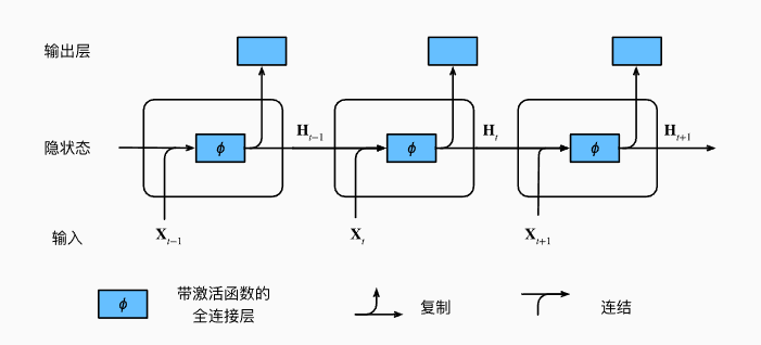
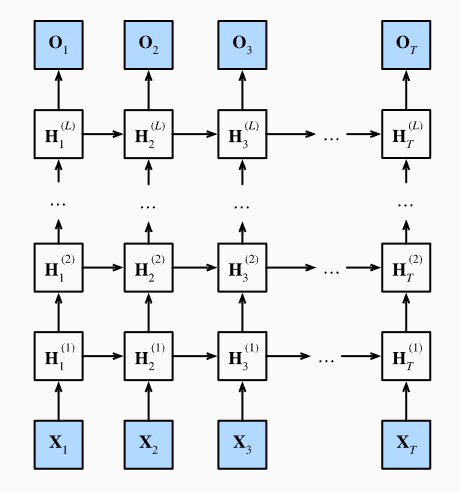
- RNN结构
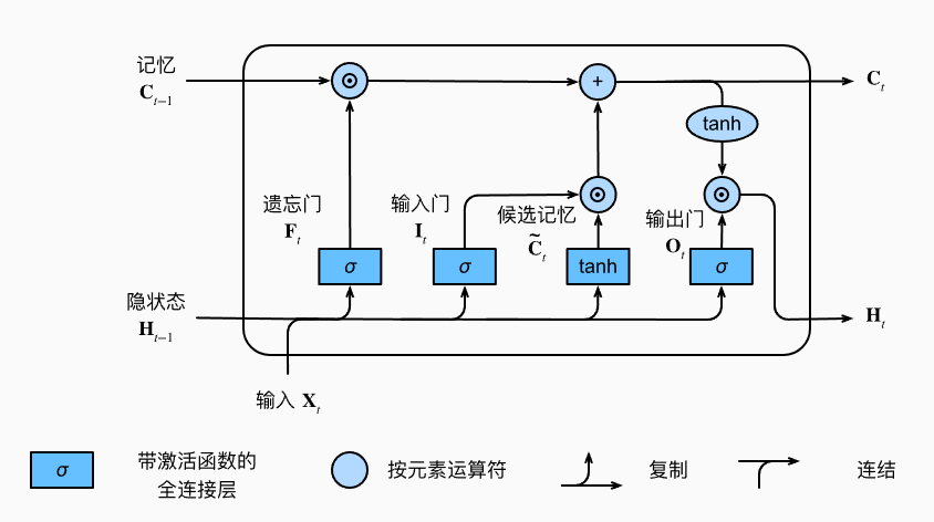
- LSTM结构
- 样本和标签
- 2 Transformer
- transformer结构
- 位置编码
1 RNN & LSTM
RNN结构
LSTM结构
代码(使用CPU):
import numpy as np
import torch
from matplotlib import pyplot as plt
from torch import nn
import pandas as pd
from sklearn import preprocessing
import torch.utils.data
import torch.utils.data as Data
from sklearn.metrics import mean_squared_error  # MSE
from sklearn.metrics import mean_absolute_error  # MAE
# 1. 读取csv表格数据.使用4000个数据点
data = pd.read_csv('data/pollution.csv').values[6000:10000]  # numpy.ndarray# 2. 选取 pollution, dew, temp, press 作为我们要学习和预测的数据
data = data[:, [1, 2, 3, 4]]
plt.plot(data)
plt.title('Pollution Data Visualization')
plt.xlabel('Time Steps')
plt.ylabel('Values')
plt.legend(['Pollution', 'Dew Point', 'Temperature', 'Pressure'])  # 根据数据列名添加图例
plt.show()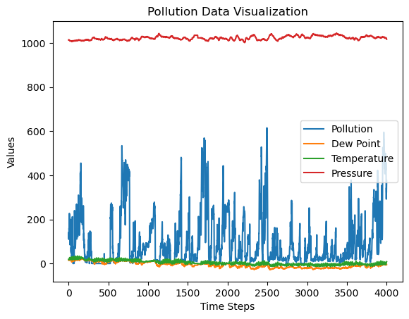
# 3. 数据归一化。按均值和方差将数据限制在[-1,1]或者[0,1]
min_max_scaler = preprocessing.MinMaxScaler()
data = min_max_scaler.fit_transform(data)
样本和标签
# 设置样本和标签 样本1:(x_0,x_1,...x_n-1) -> 标签1:(x_1,x_2,...x_n),
#               样本2:(x_1,x_2,...x_n) -> 标签2:(x_2,x_3,...x_n+1) ,...
# 让模型基于输入的前一组观测值预测接下来的一组观测值,想达到的效果为根据一组时间步观测值预测后面一步的观测值
WINDOW_SIZE = 50
samples = []
labels = []
for i in range(len(data) - WINDOW_SIZE):samples.append(data[i:i + WINDOW_SIZE])labels.append(data[i + 1:i + WINDOW_SIZE + 1])
samples = torch.tensor(np.array(samples), dtype=torch.float32)
labels = torch.tensor(np.array(labels), dtype=torch.float32)
# 4. 划分训练集,测试集 按4:1划分
train_test_boundary = int(len(data) * 0.8)
train_samples = samples[:train_test_boundary, :] # torch.Size([3200, 50, 4]),即3200个样本,每个样本有50个时间步,每个时间步有4个特征
train_labels = labels[:train_test_boundary, :] # torch.Size([3200, 50, 4])
test_samples = samples[train_test_boundary:, :] # torch.Size([750, 50, 4])
# 5. 使用pytorch的dataloader构建数据集
BATCH_SIZE = 32
train_dataset = Data.TensorDataset(train_samples, train_labels)
train_loader = Data.DataLoader(dataset=train_dataset, batch_size=BATCH_SIZE, shuffle=True)
# 打乱操作仅发生在样本之间,而不是样本内部。即,每个样本本身的时间序列(窗口)是保持不变的。
# 模型的定义
# RNN类定义
class RNN(nn.Module):def __init__(self, series_dim, hidden_size, num_layers):# series_dim: 输入数据的维度,即每个时间步的数据特征数super(RNN, self).__init__()self.hidden_size = hidden_sizeself.num_layers = num_layersself.rnn = nn.RNN(series_dim, hidden_size, num_layers, batch_first=True)self.linear = nn.Linear(hidden_size, series_dim)def __call__(self, input, state): # 自动调用forward方法# input: (batch_size, seq_len, series_dim)hiddens, outputs = self.rnn(input, state)return self.linear(hiddens)def init_state(self, batch_size):return torch.zeros((self.num_layers, batch_size, self.hidden_size))# LSTM类定义
class LSTM(nn.Module):def __init__(self, series_dim, hidden_size, num_layers):super(LSTM, self).__init__()self.hidden_size = hidden_sizeself.num_layers = num_layersself.lstm = nn.LSTM(series_dim, hidden_size, num_layers, batch_first=True)self.linear = nn.Linear(hidden_size, series_dim)def __call__(self, input, state):hiddens, (h_n, c_n) = self.lstm(input, state)return self.linear(hiddens)def init_state(self, batch_size):h0 = torch.zeros(self.num_layers, batch_size, self.hidden_size, requires_grad=True)c0 = torch.zeros(self.num_layers, batch_size, self.hidden_size, requires_grad=True)return (h0, c0)
# 6. 实例化模型
TIME_SERIES_DIM = 4
HIDDEN_SIZE = 64
NUM_LAYERS = 2
model1 = LSTM(TIME_SERIES_DIM, HIDDEN_SIZE, NUM_LAYERS)
model2 = RNN(TIME_SERIES_DIM, HIDDEN_SIZE, NUM_LAYERS)# 7. 定义损失函数和优化器等
LEARNING_RATE = 0.001
loss_function1 = nn.MSELoss()
loss_function2 = nn.MSELoss()
updater1 = torch.optim.Adam(model1.parameters(), LEARNING_RATE)
updater2 = torch.optim.Adam(model2.parameters(), LEARNING_RATE)
# 8. 开始训练
EPOCH = 10
loss_lstm = []
loss_rnn = []
for epoch in range(EPOCH):current_epoch_loss1 = 0current_epoch_loss2 = 0for X, Y in train_loader:# 循环神经网络初始化状态state1 = model1.init_state(BATCH_SIZE)state2 = model2.init_state(BATCH_SIZE)# 把当前状态state和当前输入X输入进模型Y_pred1 = model1(X, state1)Y_pred2 = model2(X, state2)# 通过损失函数和优化器来更新updater1.zero_grad()updater2.zero_grad()loss1 = loss_function1(Y_pred1, Y) # 返回的是一个batch里的平均损失loss2 = loss_function2(Y_pred2, Y)current_epoch_loss1 += loss1.item()  # 使用 item() 获取当前 batch 的损失current_epoch_loss2 += loss2.item()loss1.backward()loss2.backward()updater1.step()  # 梯度下降更新权重updater2.step()loss_lstm.append(current_epoch_loss1)loss_rnn.append(current_epoch_loss2)print(f"*Current epoch:{epoch} lstm'training loss:{current_epoch_loss1} rnn'training loss:{current_epoch_loss2}")
*Current epoch:0 lstm'training loss:3.9102106178179383 rnn'training loss:1.8705139216035604
*Current epoch:1 lstm'training loss:0.9454482225701213 rnn'training loss:0.31060056993737817
*Current epoch:2 lstm'training loss:0.535230312962085 rnn'training loss:0.19003595446702093
*Current epoch:3 lstm'training loss:0.35580030153505504 rnn'training loss:0.14062378648668528
*Current epoch:4 lstm'training loss:0.2430544177768752 rnn'training loss:0.11611037276452407
*Current epoch:5 lstm'training loss:0.17943283065687865 rnn'training loss:0.10188076680060476
*Current epoch:6 lstm'training loss:0.14488379610702395 rnn'training loss:0.09293708164477721
*Current epoch:7 lstm'training loss:0.12210956087801605 rnn'training loss:0.08662866713711992
*Current epoch:8 lstm'training loss:0.10986834816867486 rnn'training loss:0.08307236654218286
*Current epoch:9 lstm'training loss:0.10131064016604796 rnn'training loss:0.0803355200914666
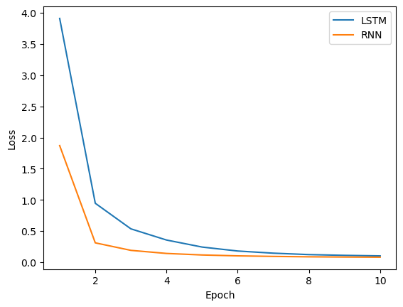
# 画出损失函数的变化
plt.plot(np.arange(1,EPOCH+1),loss_lstm, label='LSTM')
plt.plot(np.arange(1,EPOCH+1),loss_rnn, label='RNN')
plt.xlabel('Epoch')
plt.ylabel('Loss')
plt.legend()
plt.show()
# 9. 预测
predicted_data1 = []
predicted_data2 = []
for test_sample in test_samples: # 一个一个样本进行预测state1 = model1.init_state(batch_size=1)state2 = model2.init_state(batch_size=1)predicted_label1 = model1(test_sample.reshape(1, test_sample.shape[0], -1), state1)predicted_label2 = model2(test_sample.reshape(1, test_sample.shape[0], -1), state2)# print(predicted_label1.shape) # torch.Size([1, 50, 4])# 在测试集上进行预测时选取每次预测出的向量的最后一个点predicted_data1.append(predicted_label1[0][-1].detach().numpy())predicted_data2.append(predicted_label2[0][-1].detach().numpy())
predicted_data1 = np.array(predicted_data1) # (750, 4)
predicted_data2 = np.array(predicted_data2) # (750, 4)
# 10. 计算误差并绘制预测结果
true_data = data[train_test_boundary + WINDOW_SIZE:]
MSE1 = mean_squared_error(true_data, predicted_data1)
MSE2 = mean_squared_error(true_data, predicted_data2)
MAE1 = mean_absolute_error(true_data, predicted_data1)
MAE2 = mean_absolute_error(true_data, predicted_data2)
print(f"LSTM'MSE:{round(MSE1, 5)} MAE:{round(MAE1, 5)}")
print(f"RNN'MSE:{round(MSE2, 5)} MAE:{round(MAE2, 5)}")
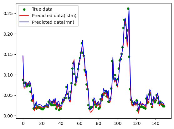
# 绘制测试集前150个时间步的预测效果
plt.scatter(np.arange(0,150),true_data[:150, 0], color = 'g',s= 20,label='True data')
plt.plot(predicted_data1[:150, 0], color = 'r',label='Predicted data(lstm)')
plt.plot(predicted_data2[:150, 0], color = 'b',label='Predicted data(rnn)')
plt.legend()
plt.show()
LSTM'MSE:0.00099 MAE:0.01979
RNN'MSE:0.00098 MAE:0.01943
2 Transformer
transformer结构
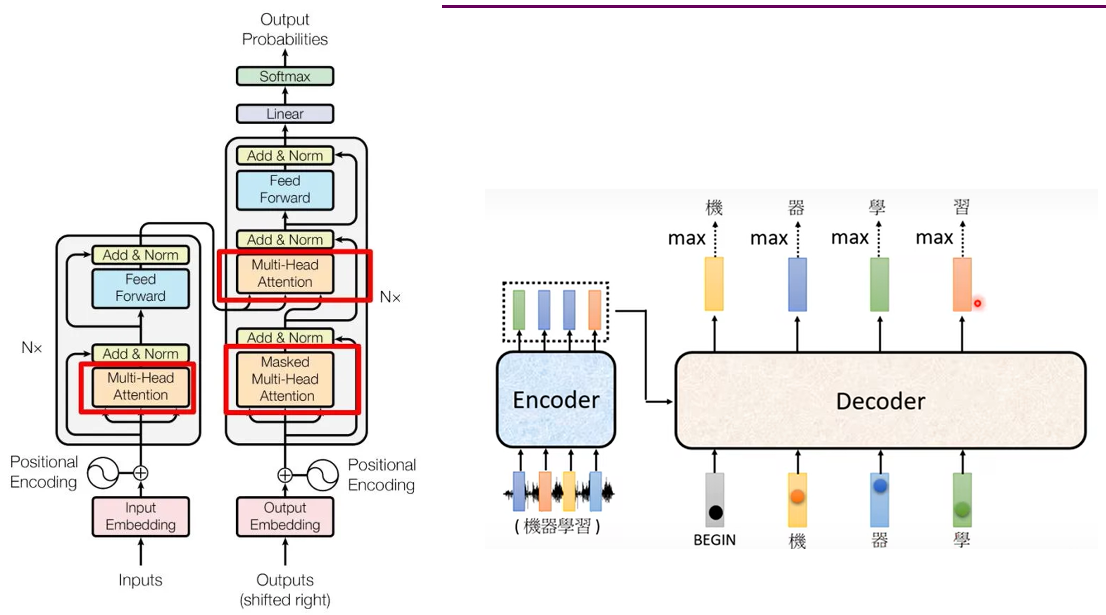
位置编码
PosEncoder ( p o s , 2 i ) = s i n ( p o s / 1000 0 2 i / d m o d e l ) P o s E n c o d e r ( p o s , 2 i + 1 ) = c o s ( p o s / 1000 0 2 i / d m o d e l ) \text{PosEncoder}(pos, 2i) = sin(pos/10000^{2i/d_{model}}) \\ {PosEncoder}(pos, 2i+1) = cos(pos/10000^{2i/d_{model}}) PosEncoder(pos,2i)=sin(pos/100002i/dmodel)PosEncoder(pos,2i+1)=cos(pos/100002i/dmodel)
其中, p o s pos pos指在一个样本中(共50个时间步)的时间步位置,这里的 2 i 2i 2i和 2 i + 1 2i+1 2i+1是特征所在位置, d m o d e l d_{model} dmodel值嵌入向量维度。
代码(使用GPU和CPU均能运行):
import numpy as np
import math
import torch
from matplotlib import pyplot as plt
from torch import nn
import pandas as pd
from sklearn import preprocessing
import torch.utils.data
import torch.utils.data as Data
import time
# 位置编码
class PositionalEncoding(nn.Module):def __init__(self, d_model, dropout=0.1, max_len=5000):super(PositionalEncoding, self).__init__()self.dropout = nn.Dropout(p=dropout)pe = torch.zeros(max_len, d_model)position = torch.arange(0, max_len, dtype=torch.float).unsqueeze(1) # 生成位置索引的列向量div_term = torch.exp(torch.arange(0, d_model, 2).float() * (-math.log(10000.0) / d_model))pe[:, 0::2] = torch.sin(position * div_term)pe[:, 1::2] = torch.cos(position * div_term)pe = pe.unsqueeze(0).transpose(0, 1) # 将维度调整为(1, max_len, d_model),方便后续相加self.register_buffer('pe', pe) # 将pe注册为缓冲区,以便不被视为模型的参数def forward(self, x):r"""Inputs of forward functionArgs:x: the sequence fed to the positional encoder model (required).Shape:x: [sequence length, batch size, embed dim]output: [sequence length, batch size, embed dim]Examples:>>> output = pos_encoder(x)"""x = x + self.pe[:x.size(0), :] # 将位置编码加到输入的嵌入向量上return self.dropout(x)
class TransAm(nn.Module):def __init__(self, series_dim, feature_size=250, num_encoder_layers=1, num_decoder_layers=1, dropout=0.1):'''series_dim: 输入数据的维度,即时间序列数据的特征数量feature_size: 将输入嵌入到更高维空间的特征大小。它是 Transformer 的 d_model(特征维度),默认为 250。'''super(TransAm, self).__init__()self.model_type = 'Transformer'# nn.Embedding:适用于离散的分类索引(如词汇表中的单词索引),用于将离散值映射到连续向量# nn.Linear:适用于处理连续的实数值输入(如时间序列、图像特征等),用于将输入映射到高维特征空间self.input_embedding = nn.Linear(series_dim, feature_size)# self.src_mask = None# 掩码 tgt_mask,用于处理自回归的序列预测任务,保证模型不能看到未来的数据(即防止模型在预测时看到比当前步更后的信息)self.tgt_mask = Noneself.pos_encoder = PositionalEncoding(feature_size)self.encoder_layer = nn.TransformerEncoderLayer(d_model=feature_size, nhead=10, dropout=dropout)self.encoder = nn.TransformerEncoder(self.encoder_layer, num_layers=num_encoder_layers)self.decoder_layer = nn.TransformerDecoderLayer(d_model=feature_size, nhead=10, dropout=dropout)self.decoder = nn.TransformerDecoder(self.decoder_layer, num_layers=num_decoder_layers)# 将模型的输出转换回原来的时间序列维度 (series_dim),用来生成最终的预测结果self.linear1 = nn.Linear(feature_size, feature_size//2)self.linear2 = nn.Linear(feature_size//2, series_dim)def forward(self, src, tgt):'''src: 输入给编码器的序列数据(原始时间序列)。[96, 32, 7] (seq, bz, series_dim)tgt: 输入给解码器的数据,通常是部分已知的时间序列数据或初始化的解码输入。[144, 32, 7]后文这一行代码调用了forward函数:Y_pred = model(X, decoder_input) # 返回torch.Size([96, 32, 7])'''
# 在时间序列任务中,通常不需要使用 padding_mask,尤其是在处理固定长度的输入时(例如 WINDOW_SIZE 和 PREDICT_SIZE 已经定义了固定的序列长度)
# padding_mask 通常用于自然语言处理任务中,因为句子长度不同,需要在短句的末尾进行填充,而时间序列数据通常是连续的、固定长度的,不需要填充。
#         # 这个条件确保padding_mask只在首次或当输入序列长度变化时生成
#         # 编码器中的掩码是用来忽略填充部分,使得模型只关注实际的数据。
#         if self.src_mask is None or self.src_mask.size(0) != len(src):
#             device = src.device
#             # 生成一个大小为 len(src) x len(src) 的掩码矩阵
#             mask = self._generate_padding_mask(len(src)).to(device) # 因为这里是时序任务,所以_generate_padding_mask没有进行编写
#             self.src_mask = masksrc = self.input_embedding(src)src = self.pos_encoder(src)memory = self.encoder(src)#, self.src_mask) # 这里编码器不需要掩码# print('encoder output shape:',memory.shape) # torch.Size([96, 32, 250])# 对decoder输入进行位置编码,输入decodertgt = self.input_embedding(tgt)tgt = self.pos_encoder(tgt)# print(tgt.shape) # torch.Size([144, 32, 250])# 生成解码器的掩码if self.tgt_mask is None or self.tgt_mask.size(0) != len(tgt):device = tgt.devicetgt_mask = self._generate_square_subsequent_mask(len(tgt)).to(device)self.tgt_mask = tgt_maskoutput = self.decoder(tgt, memory, tgt_mask=self.tgt_mask) # 接受目标序列的 tgt 、编码器输出的 memory和掩码tgt_mask,通过交叉注意力机制解码出新的输出# print('decoder output shape:',output.shape) # torch.Size([144, 32, 250])# 结果连一个线性层output = self.linear1(output) output = self.linear2(nn.functional.relu(output)) # torch.Size([144, 32, 7])# 结果抛去历史部分,只把要预测PREDICT_SIZE步的结果提取出来return output[-PREDICT_SIZE:, :, :]def _generate_square_subsequent_mask(self, sz):'''生成一个上三角掩码矩阵,防止模型在预测时看到未来时间步的数据。若 sz = 4 则生成:[[0.0,   -inf,  -inf,  -inf],[0.0,    0.0,  -inf,  -inf],[0.0,    0.0,   0.0,  -inf],[0.0,    0.0,   0.0,   0.0]]'''mask = (torch.triu(torch.ones(sz, sz)) == 1).transpose(0, 1)mask = mask.float().masked_fill(mask == 0, float('-inf')).masked_fill(mask == 1, float(0.0))return mask
DEVICE = torch.device("cuda:0" if torch.cuda.is_available() else "cpu")
# 准备进行数据的处理(划分样本和标签,训练集与测试集的划分)
data = pd.read_csv('/kaggle/input/example-dataset/ETTh1.csv').values[0:10000]
data = data[:, 1:] # 去掉日期列,得到7列特征
# plt.plot(data)
# plt.show()
# 数据归一化:按均值和方差将数据限制在[-1,1]或者[0,1]
min_max_scaler = preprocessing.MinMaxScaler()
data = min_max_scaler.fit_transform(data)
BATCH_SIZE = 32
# 构建样本与标签
WINDOW_SIZE = 96 # 表示样本的窗口大小,每个样本将包含 96 个时间步的数据
LABEL_SIZE = 48 # 表示标签中历史部分的大小,模型在预测时会使用这部分作为已知数据进行预测。(这里其实就是一个样本中(共96个时间步)的后48个时间步)
PREDICT_SIZE = 96 # 表示要预测的未来时间步的数量,模型将预测 96 个时间步的未来数据。
samples = [] # 存储从原始数据 data 中提取的样本(窗口),每个样本的长度为 WINDOW_SIZE。
labels = [] # 存储与每个样本对应的标签,标签由 LABEL_SIZE 和 PREDICT_SIZE 组成,包含模型需要预测的部分数据。
for i in range(len(data) - WINDOW_SIZE - PREDICT_SIZE): # 共len(data) - WINDOW_SIZE - PREDICT_SIZE个样本samples.append(data[i:i + WINDOW_SIZE]) # 最后一个样本的最后一行在data中的索引为len(data) - PREDICT_SIZE -2# 标签从 i + WINDOW_SIZE - LABEL_SIZE 开始,到 i + WINDOW_SIZE + PREDICT_SIZE-1 为止。这部分包含了历史部分(LABEL_SIZE)和未来预测部分(PREDICT_SIZE)# 即一个样本的seq_len = WINDOW_SIZE,但是该样本对应标签的seq_len可不是WINDOW_SIZE,而是LABEL_SIZE + PREDICT_SIZElabels.append(data[i + WINDOW_SIZE - LABEL_SIZE:i + WINDOW_SIZE + PREDICT_SIZE])# 最后一个标签的最后一行在data中的索引为len(data) -2
samples = torch.tensor(np.array(samples), dtype=torch.float32) # 9808个样本
labels = torch.tensor(np.array(labels), dtype=torch.float32) # 9808个标签# 划分训练集,测试集 按4:1划分
train_test_boundary = int(len(data) * 0.8) # 8000
train_samples = samples[:train_test_boundary, :].to(DEVICE) # 8000
train_labels = labels[:train_test_boundary, :].to(DEVICE) # 8000
test_samples = samples[train_test_boundary:, :].to(DEVICE) # 1808
test_labels = labels[train_test_boundary:, :].to(DEVICE) # 1808# 使用pytorch的dataloader构建数据集
train_dataset = Data.TensorDataset(train_samples, train_labels)
train_loader = Data.DataLoader(dataset=train_dataset, batch_size=BATCH_SIZE, shuffle=True)
LEARNING_RATE = 0.001
EPOCH = 20
# 数据已准备好,开始训练
# 实例化模型,这里使用Transformer作为我们的模型. 这里feature_size=100。前文注释写的250,懒得改了
model = TransAm(series_dim=7,feature_size=100,num_encoder_layers=1, num_decoder_layers=1)
model = model.to(DEVICE)# 定义损失函数和优化器等
loss_function = nn.MSELoss()
updater = torch.optim.Adam(model.parameters(), LEARNING_RATE)# 开始训练
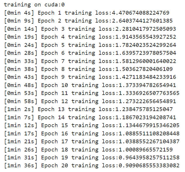
def train():print(f'training on {DEVICE}')start = time.time()for epoch in range(EPOCH):current_epoch_loss = 0for X, Y in train_loader: # X 和 Y 的维度:(batch_size, sequence_length, series_dim),torch.Size([32, 96, 7]) torch.Size([32, 144, 7])# 把数据的第0维和第1维转一下,即把输入和输出转为 (sequence_length, batch_size, series_dim)的格式X, Y = X.permute(1, 0, 2), Y.permute(1, 0, 2)decoder_input = torch.zeros_like(Y[-PREDICT_SIZE:, :, :]).float() # # torch.Size([96, 32, 7])# 将 LABEL_SIZE 的历史数据部分与零初始化的未来部分拼接起来,形成解码器的完整输入# 可以发现Y[:LABEL_SIZE, :, ]其实就等于X[-LABEL_SIZE:,:,:]decoder_input = torch.cat([X[-LABEL_SIZE:,:,:], decoder_input], dim=0).float().to(DEVICE) # torch.Size([144, 32, 7])Y_pred = model(X, decoder_input) # torch.Size([96, 32, 7]) # 效果为:用48个历史时间步数据预测了未来96个时间步updater.zero_grad()loss = loss_function(Y_pred, Y[-PREDICT_SIZE:, :, :]) # loss形如tensor(0.3840, device='cuda:0', grad_fn=<MseLossBackward0>)loss.backward()current_epoch_loss+=loss.item()updater.step() # 梯度下降更新权重print(f'[{timeSince(start)}] Epoch {epoch+1} ', end='')print(f"training loss:{current_epoch_loss}")
# torch.save(model.state_dict(), 'model.pt')
def timeSince(since):now = time.time()s = now - sincem = math.floor(s / 60) # math.floor()向下取整s -= m * 60return '%dmin %ds' % (m, s)
MODEL_SAVED = False
if MODEL_SAVED: # 若为True.先实例化模型 model = TransAm(series_dim=7),再加载已保存好的模型model.load_state_dict(torch.load('model.pt'))
else:train()
from matplotlib_inline import backend_inline
backend_inline.set_matplotlib_formats('svg')
# 预测
# 设置 BATCH_SIZE 为1,即一次预测一个样本,要达到的效果为:根据一个样本中最后48个历史数据去预测未来96个数据
test_input = test_samples[400].reshape(WINDOW_SIZE, 1, 7)
test_output = test_labels[400].reshape(PREDICT_SIZE + LABEL_SIZE, 1, 7) # 该样本对应的标签
decoder_input = torch.zeros_like(test_output[-PREDICT_SIZE:, :, :]).float()
decoder_input = torch.cat([test_input[-LABEL_SIZE:, :, :], decoder_input], dim=0).float().to(DEVICE)
prediction = model(test_input, decoder_input)
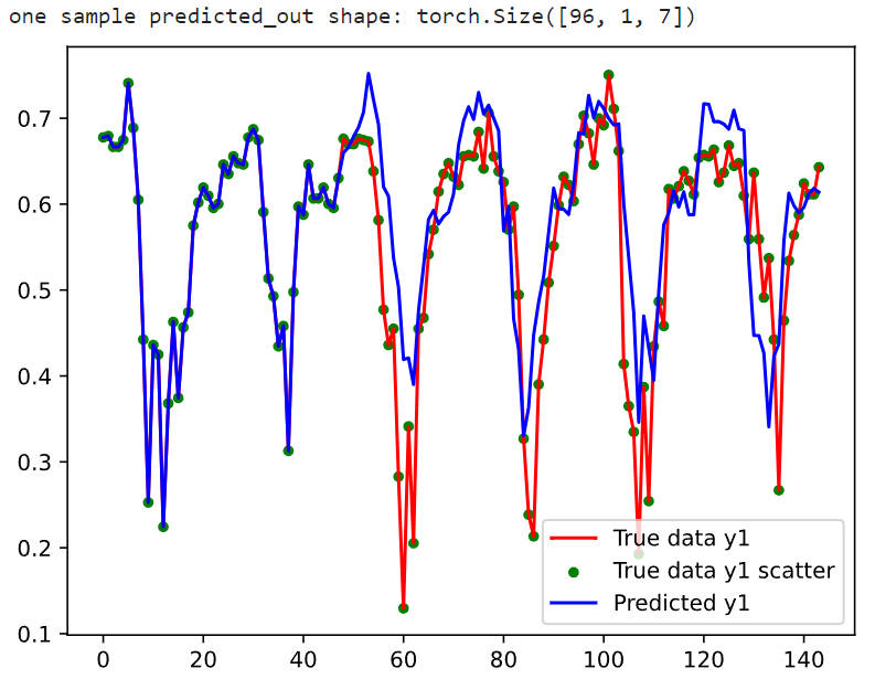
print('one sample predicted_out shape:',prediction.shape)# 绘制
true_output = test_output.cpu().numpy().reshape(PREDICT_SIZE + LABEL_SIZE, 7) # (144, 7)
predict_output = prediction.detach().cpu().numpy().reshape(PREDICT_SIZE, 7) # (96,7)
predict_output = np.concatenate((true_output[:LABEL_SIZE], predict_output), axis=0) # (144,7)
plt.plot(true_output[:, 0], color = 'r',label='True data y1')
plt.scatter(np.arange(0,PREDICT_SIZE + LABEL_SIZE),true_output[:, 0], color = 'g',s= 15,label='True data y1 scatter')
plt.plot(predict_output[:, 0], color = 'b',label='Predicted y1')
plt.legend()
plt.show()
代码参考:https://gitee.com/encorew/time-series-practice