——欲速则不达,我已经很幸运了,只要珍惜这份幸运就好了,不必患得患失,慢慢来。
----查漏补缺:
1.关于这个os.listdir的使用

2.从‘num_文件名.jpg’中提取出数值:

3.slic图像分割标记函数的作用:

4.zip这个函数,用来讲2个数组“一一对应”的合成1个数组:

5.关于astype的这个用来类型转换的东西:

6.关于 利用[]合并之后,再进行enumerate:

PART1:11个food的分类问题的explainable部分:
一、对于这个cnn的代码部分的回顾:
1.前期准备:库的引入,参数的设置
import os
import sys
import argparse
import numpy as np
from PIL import Image
import matplotlib.pyplot as plt
import torch
import torch.nn as nn
import torch.nn.functional as F
from torch.optim import Adam
from torch.utils.data import Dataset
import torchvision.transforms as transforms
from skimage.segmentation import slic
from lime import lime_image
from pdb import set_trace
from torch.autograd import Variable
args = {'ckptpath': './checkpoint.pth','dataset_dir': './food/'
}
args = argparse.Namespace(**args)2.模型结构的定义:
(1)cnn是一系列的卷积层最终得到4**4*512的图像
(2)flatten展平之后,再经过一系列的linear层得到11种的向量
# Model definition——分析这个model的结构:class Classifier(nn.Module):def __init__(self):super(Classifier, self).__init__()def building_block(indim, outdim):return [nn.Conv2d(indim, outdim, 3, 1, 1),nn.BatchNorm2d(outdim),nn.ReLU(),]def stack_blocks(indim, outdim, block_num):layers = building_block(indim, outdim)for i in range(block_num - 1):layers += building_block(outdim, outdim)layers.append(nn.MaxPool2d(2, 2, 0))return layerscnn_list = []cnn_list += stack_blocks(3, 128, 3)cnn_list += stack_blocks(128, 128, 3)cnn_list += stack_blocks(128, 256, 3)cnn_list += stack_blocks(256, 512, 1)cnn_list += stack_blocks(512, 512, 1)self.cnn = nn.Sequential( * cnn_list) #上面所有的函数,都是为了这个cnn的过程的设计dnn_list = [nn.Linear(512 * 4 * 4, 1024),nn.ReLU(),nn.Dropout(p = 0.3),nn.Linear(1024, 11),]self.fc = nn.Sequential( * dnn_list)def forward(self, x):out = self.cnn(x)out = out.reshape(out.size()[0], -1)return self.fc(out)模型对象的实例化:
# Load trained model
model = Classifier().cuda()
checkpoint = torch.load(args.ckptpath)
model.load_state_dict(checkpoint['model_state_dict'])
# It should display: <All keys matched successfully>
3.定义food_dataset,虽然实例的部分使用eval不是很确定是不是已经把model已经train好了,还是说,只是使用eval版本的eval:
# It might take some time, if it is too long, try to reload it.
# Dataset definition
#定义这个dataset了
class FoodDataset(Dataset):def __init__(self, paths, labels, mode):# mode: 'train' or 'eval'self.paths = pathsself.labels = labelstrainTransform = transforms.Compose([transforms.Resize(size=(128, 128)),transforms.RandomHorizontalFlip(),transforms.RandomRotation(15),transforms.ToTensor(),])evalTransform = transforms.Compose([transforms.Resize(size=(128, 128)),transforms.ToTensor(),])self.transform = trainTransform if mode == 'train' else evalTransform# pytorch dataset classdef __len__(self):return len(self.paths)def __getitem__(self, index):X = Image.open(self.paths[index])X = self.transform(X)Y = self.labels[index]return X, Y# help to get images for visualizingdef getbatch(self, indices):images = []labels = []for index in indices:image, label = self.__getitem__(index)images.append(image)labels.append(label)return torch.stack(images), torch.tensor(labels)# help to get data path and label
#先分析这个函数,再分析上面的dataset
def get_paths_labels(path):#定义1个lambda函数def my_key(name):return int(name.replace(".jpg",""))+1000000*int(name.split("_")[0])imgnames = os.listdir(path)imgnames.sort(key=my_key) #使用这个lambda函数进行sort排序imgpaths = []labels = []for name in imgnames:imgpaths.append(os.path.join(path, name))labels.append(int(name.split('_')[0]))return imgpaths, labels
train_paths, train_labels = get_paths_labels(args.dataset_dir)  #没问题,只是key处理了,但是name本身没改变train_set = FoodDataset(train_paths, train_labels, mode='eval') #可能这里用到的model是已经train好的model
从这个dataset中抽出11张图像进行人工观察:
img_indices = [i for i in range(10)]
images, labels = train_set.getbatch(img_indices)
fig, axs = plt.subplots(1, len(img_indices), figsize=(15, 8))
for i, img in enumerate(images):axs[i].imshow(img.cpu().permute(1, 2, 0))
# print(labels)
二、使用Lime对图像中的
1.Local Interpretable Model-Agnostic Explanations的定义:

2.具体使用这个lime:
#调用model的eval对整个batch的input进行预测得到1个batch的predicts结果
def predict(input):# input: numpy array, (batches, height, width, channels)                                                                                                                                                     model.eval()                                                                                                                                                             input = torch.FloatTensor(input).permute(0, 3, 1, 2)                                                                                                            # pytorch tensor, (batches, channels, height, width)output = model(input.cuda())                                                                                                                                             return output.detach().cpu().numpy()                                                                                                                              #对输入的图像进行分割后标记
def segmentation(input):# split the image into 200 pieces with the help of segmentaion from skimage                                                                                                                   return slic(input, n_segments=200, compactness=1, sigma=1)                                                                                                              #设置画布参数
fig, axs = plt.subplots(1, len(img_indices), figsize=(15, 8))
# fix the random seed to make it reproducible
np.random.seed(16)    for idx, (image, label) in enumerate(zip(images.permute(0, 2, 3, 1).numpy(), labels)):                                                                                                                                             x = image.astype(np.double)# numpy array for lime#调用explainer的explain_instance,传递对应图像x,predict函数,segmentation函数作为它的参数explainer = lime_image.LimeImageExplainer()                                                                                                                              explaination = explainer.explain_instance(image=x, classifier_fn=predict, segmentation_fn=segmentation)# doc: https://lime-ml.readthedocs.io/en/latest/lime.html?highlight=explain_instance#lime.lime_image.LimeImageExplainer.explain_instance#调用上面的这个explaination,传递的参数主要是label值 和 num_features种类,其他的就是说是否显示不是重要的地方等。。lime_img, mask = explaination.get_image_and_mask(                                                                                                                         label=label.item(),                                                                                                                           positive_only=False,                                                                                                                         hide_rest=False,                                                                                                                             num_features=11,                                                                                                                              min_weight=0.05                                                                                                                              )# turn the result from explainer to the image# doc: https://lime-ml.readthedocs.io/en/latest/lime.html?highlight=get_image_and_mask#lime.lime_image.ImageExplanation.get_image_and_maskaxs[idx].imshow(lime_img) #axs的第idx位置的图像,就放置这个lime_img了#show出这些用lime标记的图像咯
plt.show()
plt.close()
三、使用saliency map:显著性标注出这个图像中贡献这个类型特征最多的地方
(其实就是普通的gradient的方法)
The heatmaps that highlight pixels of the input image that contribute the most in the classification task.
总的来说,就是通过计算每个pixel对于整个loss的gradient,这个gradient就是新的图像的pixel数值
#对图像中的每个pixel的数值进行normalize
def normalize(image):return (image - image.min()) / (image.max() - image.min())# return torch.log(image)/torch.log(image.max())#用于计算saliency的函数
def compute_saliency_maps(x, y, model): #x就是图像, y就是label, model就是分类器model.eval()x = x.cuda()# we want the gradient of the input xx.requires_grad_()y_pred = model(x)loss_func = torch.nn.CrossEntropyLoss()loss = loss_func(y_pred, y.cuda())loss.backward()# saliencies = x.grad.abs().detach().cpu()saliencies, _ = torch.max(x.grad.data.abs().detach().cpu(),dim=1) #这一步,就是将每个像素的位置的gradient梯度(3个通道中的最大的那个)作为新的图像位置的 像素值# We need to normalize each image, because their gradients might vary in scale, but we only care about the relation in each imagesaliencies = torch.stack([normalize(item) for item in saliencies])return saliencies
# images, labels = train_set.getbatch(img_indices)
saliencies = compute_saliency_maps(images, labels, model)# visualize
fig, axs = plt.subplots(2, len(img_indices), figsize=(15, 8))
for row, target in enumerate([images, saliencies]):for column, img in enumerate(target):if row==0:axs[row][column].imshow(img.permute(1, 2, 0).numpy()) #第一行:正常图像显示# What is permute?# In pytorch, the meaning of each dimension of image tensor is (channels, height, width)# In matplotlib, the meaning of each dimension of image tensor is (height, width, channels)# permute is a tool for permuting dimensions of tensors# For example, img.permute(1, 2, 0) means that,# - 0 dimension is the 1 dimension of the original tensor, which is height# - 1 dimension is the 2 dimension of the original tensor, which is width# - 2 dimension is the 0 dimension of the original tensor, which is channelselse:axs[row][column].imshow(img.numpy(), cmap=plt.cm.hot) #第二行:热成像图plt.show()
plt.close()四、smooth grad的方法查看heat 图像
Smooth grad
Smooth grad 的方法是,在圖片中隨機地加入 noise,然後得到不同的 heatmap,把這些 heatmap 平均起來就得到一個比較能抵抗 noisy gradient 的結果。
# Smooth grad
#一样的normalize函数
def normalize(image):return (image - image.min()) / (image.max() - image.min())#计算出类似于saliency map中的saliencies图像的东西:
def smooth_grad(x, y, model, epoch, param_sigma_multiplier):         #总共epoch数,一个常量sigmamodel.eval()#x = x.cuda().unsqueeze(0)mean = 0sigma = param_sigma_multiplier / (torch.max(x) - torch.min(x)).item()  #sigma就是1个数值smooth = np.zeros(x.cuda().unsqueeze(0).size())               #一个和x相同大小zero变量for i in range(epoch):# call Variable to generate random noisenoise = Variable(x.data.new(x.size()).normal_(mean, sigma**2))     #sigma用作正太分布的标准差参数,抽取noise的抽样,和x一样大x_mod = (x+noise).unsqueeze(0).cuda()x_mod.requires_grad_()y_pred = model(x_mod)loss_func = torch.nn.CrossEntropyLoss()loss = loss_func(y_pred, y.cuda().unsqueeze(0))loss.backward()# like the method in saliency mapsmooth += x_mod.grad.abs().detach().cpu().data.numpy()      #smooth用于累计每一个epoch的和smooth = normalize(smooth / epoch) # don't forget to normalize,取个均值就可以了# smooth = smooth / epochreturn smooth# images, labels = train_set.getbatch(img_indices)
smooth = []
for i, l in zip(images, labels):smooth.append(smooth_grad(i, l, model, 500, 0.4))
smooth = np.stack(smooth)
print(smooth.shape)fig, axs = plt.subplots(2, len(img_indices), figsize=(15, 8)) #2行喔!
for row, target in enumerate([images, smooth]):for column, img in enumerate(target):axs[row][column].imshow(np.transpose(img.reshape(3,128,128), (1,2,0)))
五、Filter Explanation,透过卷积的中间层进行观察:
1.hook钩子函数的作用:

2.只输出指定filterid的那个滤波器的输出:

3.具体的代码部分
#定义正规化
def normalize(image):return (image - image.min()) / (image.max() - image.min())layer_activations = None
#filter的观察函数,返回的是 activation 和 visulization
def filter_explanation(x, model, cnnid, filterid, iteration=100, lr=1):#cnnid是对应的卷积层的id,filterid是对应的过滤器的id# x: input image# cnnid, filterid: cnn layer id, which filtermodel.eval()def hook(model, input, output): #定义hook函数,就是将output给到全局的layer_activationsglobal layer_activationslayer_activations = outputhook_handle = model.cnn[cnnid].register_forward_hook(hook)  #hook的handle句柄,下面有解释这行代码的含义# When the model forward through the layer[cnnid], need to call the hook function first# The hook function save the output of the layer[cnnid]# After forwarding, we'll have the loss and the layer activation# Filter activation: x passing the filter will generate the activation mapmodel(x.cuda()) # forward# Based on the filterid given by the function argument, pick up the specific filter's activation map# We just need to plot it, so we can detach from graph and save as cpu tensorfilter_activations = layer_activations[:, filterid, :, :].detach().cpu()# Filter visualization: find the image that can activate the filter the mostx = x.cuda()x.requires_grad_()# input image gradientoptimizer = Adam([x], lr=lr)# Use optimizer to modify the input image to amplify filter activationfor iter in range(iteration): #iteration==100optimizer.zero_grad()model(x)objective = -layer_activations[:, filterid, :, :].sum()# We want to maximize the filter activation's summation# So we add a negative signobjective.backward()# Calculate the partial differential value of filter activation to input imageoptimizer.step()# Modify input image to maximize filter activationfilter_visualizations = x.detach().cpu().squeeze()# Don't forget to remove the hookhook_handle.remove()# The hook will exist after the model register it, so you have to remove it after used# Just register a new hook if you want to use itreturn filter_activations, filter_visualizations
images, labels = train_set.getbatch(img_indices)
#下面的这个函数的参数可以看出,是获取第cnnid==6第6个卷积层的第0个过滤器的activation和visulization
filter_activations, filter_visualizations = filter_explanation(images, model, cnnid=6, filterid=0, iteration=100, lr=0.1)#以下总共进行了3组图片的绘制,分别是原始图片、activation图片,visulation图片
fig, axs = plt.subplots(3, len(img_indices), figsize=(15, 8))
for i, img in enumerate(images):axs[0][i].imshow(img.permute(1, 2, 0))
# Plot filter activations
for i, img in enumerate(filter_activations):axs[1][i].imshow(normalize(img))
# Plot filter visualization
for i, img in enumerate(filter_visualizations):axs[2][i].imshow(normalize(img.permute(1, 2, 0)))
plt.show()
plt.close()# 從下面四張圖可以看到,activate 的區域對應到一些物品的邊界,尤其是顏色對比較深的邊界images, labels = train_set.getbatch(img_indices)
#下面的这个函数的参数可以看出,是获取第cnnid==23第23个卷积层的第0个过滤器的activation和visulization
filter_activations, filter_visualizations = filter_explanation(images, model, cnnid=23, filterid=0, iteration=100, lr=0.1)# Plot filter activations
fig, axs = plt.subplots(3, len(img_indices), figsize=(15, 8))
for i, img in enumerate(images):axs[0][i].imshow(img.permute(1, 2, 0))
for i, img in enumerate(filter_activations):axs[1][i].imshow(normalize(img))
for i, img in enumerate(filter_visualizations):axs[2][i].imshow(normalize(img.permute(1, 2, 0)))
plt.show()
plt.close()
六、使用XAI中的Integrated gradient技术:

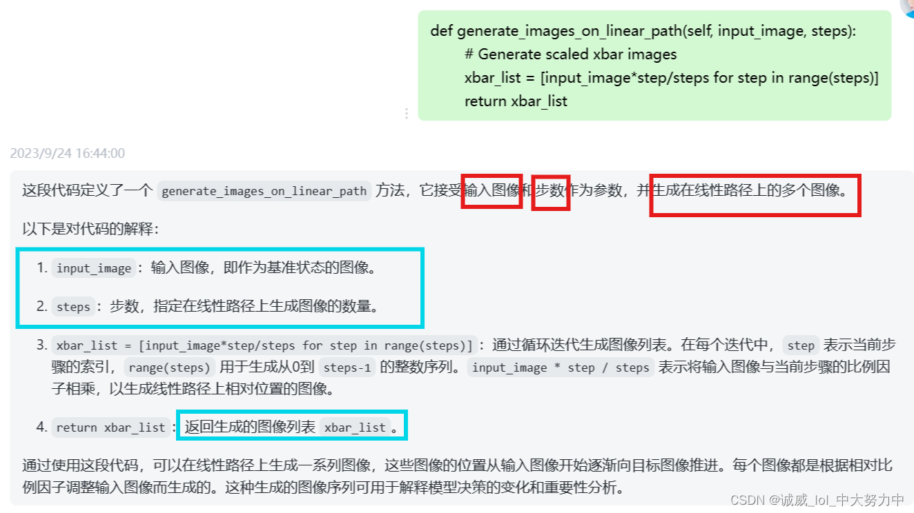
#什么都别说,5点45去西园吃点清淡的,就出去玩——看电影,或者其他的,好吧!class IntegratedGradients():def __init__(self, model): #初始化这个类self.model = modelself.gradients = None# Put model in evaluation modeself.model.eval()def generate_images_on_linear_path(self, input_image, steps):# Generate scaled xbar imagesxbar_list = [input_image*step/steps for step in range(steps)]return xbar_listdef generate_gradients(self, input_image, target_class): #计算一张图像的gradient# We want to get the gradients of the input imageinput_image.requires_grad=True# Forwardmodel_output = self.model(input_image)# Zero gradsself.model.zero_grad()# Target for backpropone_hot_output = torch.FloatTensor(1, model_output.size()[-1]).zero_().cuda()one_hot_output[0][target_class] = 1# Backwardmodel_output.backward(gradient=one_hot_output)self.gradients = input_image.grad# Convert Pytorch variable to numpy array# [0] to get rid of the first channel (1,3,128,128)gradients_as_arr = self.gradients.data.cpu().numpy()[0]return gradients_as_arrdef generate_integrated_gradients(self, input_image, target_class, steps): #计算img_list的图像的gradient的integrate# Generate xbar imagesxbar_list = self.generate_images_on_linear_path(input_image, steps)# Initialize an iamge composed of zerosintegrated_grads = np.zeros(input_image.size())for xbar_image in xbar_list:# Generate gradients from xbar imagessingle_integrated_grad = self.generate_gradients(xbar_image, target_class)# Add rescaled grads from xbar imagesintegrated_grads = integrated_grads + single_integrated_grad/steps# [0] to get rid of the first channel (1,3,128,128)return integrated_grads[0]def normalize(image):return (image - image.min()) / (image.max() - image.min())# put the image to cuda
images, labels = train_set.getbatch(img_indices)
images = images.cuda()IG = IntegratedGradients(model)
integrated_grads = []
for i, img in enumerate(images):img = img.unsqueeze(0)integrated_grads.append(IG.generate_integrated_gradients(img, labels[i], 10))
fig, axs = plt.subplots(2, len(img_indices), figsize=(15, 8))
for i, img in enumerate(images): #输出一组正常的图像axs[0][i].imshow(img.cpu().permute(1, 2, 0))
for i, img in enumerate(integrated_grads): #输出integrate的图像axs[1][i].imshow(np.moveaxis(normalize(img),0,-1))
plt.show()
plt.close()PART2:有关BERT的可解释行的model
(一)、在这个网站上感受bert的各个层的过程:
exBERT
这个模型可以用于查看注意力头部等信息,这里我就先不管了,后期慢慢摸索吧。。。。
(二)、visualizing bert's embedding:
湯姆有 3 個預訓練模型,但他忘記每一個模型是否有微調在閱讀理解的任務上了
通过观察各个token的embedding的位置,分析这个model是否具有阅读理解的fine_tune,
、。。。。我没做出来,有点难,
不过,它的代码就是从bert的每一层中取出embedding结果,再将每个token投射到二维坐标中进行分析
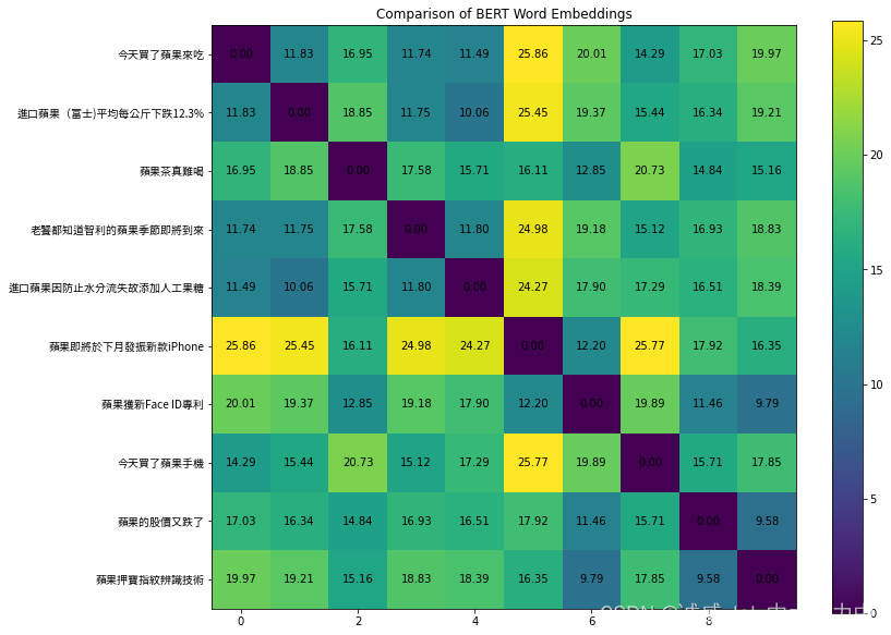
(三)、分析 吃的苹果 和 苹果手机的苹果词汇的embedding的距离
# Sentences for visualization
sentences = []
sentences += ["今天買了蘋果來吃"]
sentences += ["進口蘋果(富士)平均每公斤下跌12.3%"]
sentences += ["蘋果茶真難喝"]
sentences += ["老饕都知道智利的蘋果季節即將到來"]
sentences += ["進口蘋果因防止水分流失故添加人工果糖"]
sentences += ["蘋果即將於下月發振新款iPhone"]
sentences += ["蘋果獲新Face ID專利"]
sentences += ["今天買了蘋果手機"]
sentences += ["蘋果的股價又跌了"]
sentences += ["蘋果押寶指紋辨識技術"]# Index of word selected for embedding comparison. E.g. For sentence "蘋果茶真難喝", if index is 0, "蘋 is selected"
select_word_index = [4, 2, 0, 8, 2, 0, 0, 4, 0, 0] #设置上面的词汇数组中的"苹果"二字的index位置
#计算向量a 和 向量b的欧式距离
def euclidean_distance(a, b):# Compute euclidean distance (L2 norm) between two numpy vectors a and breturn np.linalg.norm(a-b)#计算a向量和b向量的余弦相似度cosine_similarity = (A · B) / (||A|| * ||B||)
def cosine_similarity(a, b):# Compute cosine similarity between two numpy vectors a and breturn 0# Metric for comparison. Choose from euclidean_distance, cosine_similarity
#METRIC有2个选择,要么用欧式距离 要么用余弦相似度
METRIC = euclidean_distancedef get_select_embedding(output, tokenized_sentence, select_word_index):# The layer to visualize, choose from 0 to 12LAYER = 12# Get selected layer's hidden statehidden_state = output.hidden_states[LAYER][0]# Convert select_word_index in sentence to select_token_index in tokenized sentenceselect_token_index = tokenized_sentence.word_to_tokens(select_word_index).start# Return embedding of selected wordreturn hidden_state[select_token_index].numpy()
# Tokenize and encode sentences into model's input format
tokenized_sentences = [tokenizer(sentence, return_tensors='pt') for sentence in sentences]# Input encoded sentences into model and get outputs
with torch.no_grad():outputs = [model(**tokenized_sentence) for tokenized_sentence in tokenized_sentences]#得到词汇"苹果"在各个句子中的embedding
# Get embedding of selected word(s) in sentences. "embeddings" has shape (len(sentences), 768), where 768 is the dimension of BERT's hidden state
embeddings = [get_select_embedding(outputs[i], tokenized_sentences[i], select_word_index[i]) for i in range(len(outputs))]#计算 对应 "苹果"二字的 词汇的距离
# Pairwse comparsion of sentences' embeddings using the metirc defined. "similarity_matrix" has shape [len(sentences), len(sentences)]
similarity_matrix = pairwise_distances(embeddings, metric=METRIC) #绘制这个词汇的距离
##### Plot the similarity matrix #####
plt.rcParams['figure.figsize'] = [12, 10] # Change figure size of the plot
plt.imshow(similarity_matrix) # Display an image in the plot
plt.colorbar() # Add colorbar to the plot
plt.yticks(ticks=range(len(sentences)), labels=sentences, fontproperties=myfont) # Set tick locations and labels (sentences) of y-axis
plt.title('Comparison of BERT Word Embeddings') # Add title to the plot
for (i,j), label in np.ndenumerate(similarity_matrix): # np.ndenumerate is 2D version of enumerateplt.text(i, j, '{:.2f}'.format(label), ha='center', va='center') # Add values in similarity_matrix to the corresponding position in the plot
plt.show() # Show the plot