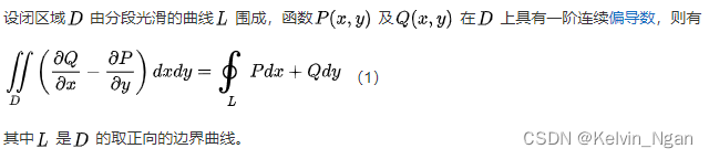
cv::contourArea计算的轮廓面积并不等于轮廓点计数，原因是cv::contourArea是基于Green公式计算

老外的讨论 github

举一个直观的例子，图中有7个像素，橙色为轮廓点连线，按照contourArea的定义，轮廓的面积为橙色所包围的区域=3

以下代码基于opencv4.8.0

cv::contourArea源码位于.\sources\modules\imgproc\src\shapedescr.cpp

// area of a whole sequence
double cv::contourArea( InputArray _contour, bool oriented )
{CV_INSTRUMENT_REGION();Mat contour = _contour.getMat();int npoints = contour.checkVector(2);int depth = contour.depth();CV_Assert(npoints >= 0 && (depth == CV_32F || depth == CV_32S));if( npoints == 0 )return 0.;double a00 = 0;bool is_float = depth == CV_32F;const Point* ptsi = contour.ptr<Point>();const Point2f* ptsf = contour.ptr<Point2f>();Point2f prev = is_float ? ptsf[npoints-1] : Point2f((float)ptsi[npoints-1].x, (float)ptsi[npoints-1].y);for( int i = 0; i < npoints; i++ ){Point2f p = is_float ? ptsf[i] : Point2f((float)ptsi[i].x, (float)ptsi[i].y);a00 += (double)prev.x * p.y - (double)prev.y * p.x;prev = p;}a00 *= 0.5;if( !oriented )a00 = fabs(a00);return a00;
}

如果计算面积需要考虑轮廓点本身，可以通过cv::drawContoursI填充轮廓获得mask图像后统计非零点个数

cv::drawContours源码位于.\sources\modules\imgproc\src\drawing.cpp，主要包括两步：收集边缘cv::CollectPolyEdges和填充边缘cv::FillEdgeCollection，How does the drawContours function work in OpenCV when a contour is filled?

struct PolyEdge
{PolyEdge() : y0(0), y1(0), x(0), dx(0), next(0) {}//PolyEdge(int _y0, int _y1, int _x, int _dx) : y0(_y0), y1(_y1), x(_x), dx(_dx) {}int y0, y1;int64 x, dx;PolyEdge *next;
};static void
CollectPolyEdges( Mat& img, const Point2l* v, int count, std::vector<PolyEdge>& edges,const void* color, int line_type, int shift, Point offset )
{int i, delta = offset.y + ((1 << shift) >> 1);Point2l pt0 = v[count-1], pt1;pt0.x = (pt0.x + offset.x) << (XY_SHIFT - shift);pt0.y = (pt0.y + delta) >> shift;edges.reserve( edges.size() + count );for( i = 0; i < count; i++, pt0 = pt1 ){Point2l t0, t1;PolyEdge edge;pt1 = v[i];pt1.x = (pt1.x + offset.x) << (XY_SHIFT - shift);pt1.y = (pt1.y + delta) >> shift;Point2l pt0c(pt0), pt1c(pt1);if (line_type < cv::LINE_AA){t0.y = pt0.y; t1.y = pt1.y;t0.x = (pt0.x + (XY_ONE >> 1)) >> XY_SHIFT;t1.x = (pt1.x + (XY_ONE >> 1)) >> XY_SHIFT;Line(img, t0, t1, color, line_type);// use clipped endpoints to create a more accurate PolyEdgeif ((unsigned)t0.x >= (unsigned)(img.cols) ||(unsigned)t1.x >= (unsigned)(img.cols) ||(unsigned)t0.y >= (unsigned)(img.rows) ||(unsigned)t1.y >= (unsigned)(img.rows)){clipLine(img.size(), t0, t1);if (t0.y != t1.y){pt0c.y = t0.y; pt1c.y = t1.y;pt0c.x = (int64)(t0.x) << XY_SHIFT;pt1c.x = (int64)(t1.x) << XY_SHIFT;}}else{pt0c.x += XY_ONE >> 1;pt1c.x += XY_ONE >> 1;}}else{t0.x = pt0.x; t1.x = pt1.x;t0.y = pt0.y << XY_SHIFT;t1.y = pt1.y << XY_SHIFT;LineAA(img, t0, t1, color);}if (pt0.y == pt1.y)continue;edge.dx = (pt1c.x - pt0c.x) / (pt1c.y - pt0c.y);if (pt0.y < pt1.y){edge.y0 = (int)(pt0.y);edge.y1 = (int)(pt1.y);edge.x = pt0c.x + (pt0.y - pt0c.y) * edge.dx; // correct starting point for clipped lines}else{edge.y0 = (int)(pt1.y);edge.y1 = (int)(pt0.y);edge.x = pt1c.x + (pt1.y - pt1c.y) * edge.dx; // correct starting point for clipped lines}edges.push_back(edge);}
}struct CmpEdges
{bool operator ()(const PolyEdge& e1, const PolyEdge& e2){return e1.y0 - e2.y0 ? e1.y0 < e2.y0 :e1.x - e2.x ? e1.x < e2.x : e1.dx < e2.dx;}
};static void
FillEdgeCollection( Mat& img, std::vector<PolyEdge>& edges, const void* color, int line_type)
{PolyEdge tmp;int i, y, total = (int)edges.size();Size size = img.size();PolyEdge* e;int y_max = INT_MIN, y_min = INT_MAX;int64 x_max = 0xFFFFFFFFFFFFFFFF, x_min = 0x7FFFFFFFFFFFFFFF;int pix_size = (int)img.elemSize();int delta;if (line_type < CV_AA)delta = 0;elsedelta = XY_ONE - 1;if( total < 2 )return;for( i = 0; i < total; i++ ){PolyEdge& e1 = edges[i];CV_Assert( e1.y0 < e1.y1 );// Determine x-coordinate of the end of the edge.// (This is not necessary x-coordinate of any vertex in the array.)int64 x1 = e1.x + (e1.y1 - e1.y0) * e1.dx;y_min = std::min( y_min, e1.y0 );y_max = std::max( y_max, e1.y1 );x_min = std::min( x_min, e1.x );x_max = std::max( x_max, e1.x );x_min = std::min( x_min, x1 );x_max = std::max( x_max, x1 );}if( y_max < 0 || y_min >= size.height || x_max < 0 || x_min >= ((int64)size.width<<XY_SHIFT) )return;std::sort( edges.begin(), edges.end(), CmpEdges() );// start drawingtmp.y0 = INT_MAX;edges.push_back(tmp); // after this point we do not add// any elements to edges, thus we can use pointersi = 0;tmp.next = 0;e = &edges[i];y_max = MIN( y_max, size.height );for( y = e->y0; y < y_max; y++ ){PolyEdge *last, *prelast, *keep_prelast;int draw = 0;int clipline = y < 0;prelast = &tmp;last = tmp.next;while( last || e->y0 == y ){if( last && last->y1 == y ){// exclude edge if y reaches its lower pointprelast->next = last->next;last = last->next;continue;}keep_prelast = prelast;if( last && (e->y0 > y || last->x < e->x) ){// go to the next edge in active listprelast = last;last = last->next;}else if( i < total ){// insert new edge into active list if y reaches its upper pointprelast->next = e;e->next = last;prelast = e;e = &edges[++i];}elsebreak;if( draw ){if( !clipline ){// convert x's from fixed-point to image coordinatesuchar *timg = img.ptr(y);int x1, x2;if (keep_prelast->x > prelast->x){x1 = (int)((prelast->x + delta) >> XY_SHIFT);x2 = (int)(keep_prelast->x >> XY_SHIFT);}else{x1 = (int)((keep_prelast->x + delta) >> XY_SHIFT);x2 = (int)(prelast->x >> XY_SHIFT);}// clip and draw the lineif( x1 < size.width && x2 >= 0 ){if( x1 < 0 )x1 = 0;if( x2 >= size.width )x2 = size.width - 1;ICV_HLINE( timg, x1, x2, color, pix_size );}}keep_prelast->x += keep_prelast->dx;prelast->x += prelast->dx;}draw ^= 1;}// sort edges (using bubble sort)keep_prelast = 0;do{prelast = &tmp;last = tmp.next;PolyEdge *last_exchange = 0;while( last != keep_prelast && last->next != 0 ){PolyEdge *te = last->next;// swap edgesif( last->x > te->x ){prelast->next = te;last->next = te->next;te->next = last;prelast = te;last_exchange = prelast;}else{prelast = last;last = te;}}if (last_exchange == NULL)break;keep_prelast = last_exchange;} while( keep_prelast != tmp.next && keep_prelast != &tmp );}
}

其中填充算法为scan-line polygon filling algorithm，下面转载该文

Polygon Filling? How do you do that?

In order to fill a polygon, we do not want to have to determine the type of polygon that we are filling. The easiest way to avoid this situation is to use an algorithm that works for all three types of polygons. Since both convex and concave polygons are subsets of the complex type, using an algorithm that will work for complex polygon filling should be sufficient for all three types. The scan-line polygon fill algorithm, which employs the odd/even parity concept previously discussed, works for complex polygon filling.

Reminder: The basic concept of the scan-line algorithm is to draw points from edges of odd parity to even parity on each scan-line.
What is a scan-line? A scan-line is a line of constant y value, i.e., y=c, where c lies within our drawing region, e.g., the window on our computer screen.

The scan-line algorithm is outlined next.

When filling a polygon, you will most likely just have a set of vertices, indicating the x and y Cartesian coordinates of each vertex of the polygon. The following steps should be taken to turn your set of vertices into a filled polygon.

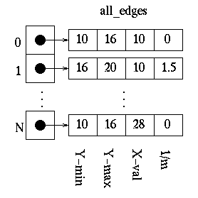
1.Initializing All of the Edges:
The first thing that needs to be done is determine how the polygon’s vertices are related. The all_edges table will hold this information.
Each adjacent set of vertices (the first and second, second and third, …, last and first) defines an edge. For each edge, the following information needs to be kept in a table:
缩进 1.The minimum y value of the two vertices.
缩进 2.The maximum y value of the two vertices.
缩进 3.The x value associated with the minimum y value.
缩进 4.The slope of the edge.
The slope of the edge can be calculated from the formula for a line:
y = mx + b;
where m = slope, b = y-intercept,
y0 = maximum y value,
y1 = minimum y value,
x0 = maximum x value,
x1 = minimum x value

The formula for the slope is as follows:
m = (y0 - y1) / (x0 - x1).

For example, the edge values may be kept as follows, where N is equal to the total number of edges - 1 and each index into the all_edges array contains a pointer to the array of edge values.

2.Initializing the Global Edge Table:
The global edge table will be used to keep track of the edges that are still needed to complete the polygon. Since we will fill the edges from bottom to top and left to right. To do this, the global edge table table should be inserted with edges grouped by increasing minimum y values. Edges with the same minimum y values are sorted on minimum x values as follows:
缩进 1.Place the first edge with a slope that is not equal to zero in the global edge table.
缩进 2.If the slope of the edge is zero, do not add that edge to the global edge table.
缩进 3.For every other edge, start at index 0 and increase the index to the global edge table once each time the current edge’s y value is greater than that of the edge at the current index in the global edge table.

Next, Increase the index to the global edge table once each time the current edge’s x value is greater than and the y value is less than or equal to that of the edge at the current index in the global edge table.

If the index, at any time, is equal to the number of edges currently in the global edge table, do not increase the index.

Place the edge information for minimum y value, maximum y value, x value, and 1/m in the global edge table at the index.

The global edge table should now contain all of the edge information necessary to fill the polygon in order of increasing minimum y and x values.

3.Initializing Parity
The initial parity is even since no edges have been crossed yet.

4.Initializing the Scan-Line
The initial scan-line is equal to the lowest y value for all of the global edges. Since the global edge table is sorted, the scan-line is the minimum y value of the first entry in this table.

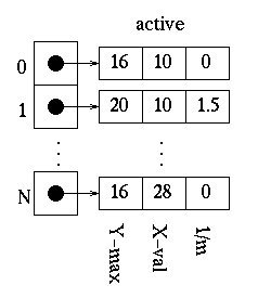
5.Initializing the Active Edge Table
The active edge table will be used to keep track of the edges that are intersected by the current scan-line. This should also contain ordered edges. This is initially set up as follows:

Since the global edge table is ordered on minimum y and x values, search, in order, through the global edge table and, for each edge found having a minimum y value equal to the current scan-line, append the edge information for the maximum y value, x value, and 1/m to the active edge table. Do this until an edge is found with a minimum y value greater than the scan line value. The active edge table will now contain ordered edges of those edges that are being filled as such:

6.Filling the Polygon
Filling the polygon involves deciding whether or not to draw pixels, adding to and removing edges from the active edge table, and updating x values for the next scan-line.

Starting with the initial scan-line, until the active edge table is empty, do the following:
缩进 1.Draw all pixels from the x value of odd to the x value of even parity edge pairs.
缩进 2.Increase the scan-line by 1.
缩进 3.Remove any edges from the active edge table for which the maximum y value is equal to the scan_line.
缩进 4.Update the x value for for each edge in the active edge table using the formula x1 = x0 + 1/m. (This is based on the line formula and the fact that the next scan-line equals the old scan-line plus one.)
缩进 5.Remove any edges from the global edge table for which the minimum y value is equal to the scan-line and place them in the active edge table.
缩进 6.Reorder the edges in the active edge table according to increasing x value. This is done in case edges have crossed.