【R语言】数据可视化分析和统计检验——线性和线性混合效应模型

R语言数据可视化分析和统计检验

写在前面
1、数据读取及分析
2、组间均值和标准差统计分析
3、图像数据探索
- 3.1 图像绘制（查看是否存在极端数据，以及数据分布情况）
- 3. 2 数据标准化（Z-scores）
- 3.3 绘制数据相关性
4、ggplot绘图
- 4.1 geom_boxplot
- 4.2 geom_dotplot()
- 4.3 geom_density
5、相关性
6、T检验
7、线性回归&ANOVA
- 7.1 绘制主效应及其交互效应
- 7.2 ANOVA
- 7.3 线性模型
- - Linear-model
8、线性混合效应模型（LMM）

写在前面

🌍✨📚最近听了北京理工大学王蓓老师关于R语言的讲座，受益匪浅，现在把自己学习的内容和收获进行记录和分享。

1、数据读取及分析

首先读取Excel数据，在这里需要对数据进行说明：该数据一共包含了5列数据，其中speaker有9类、sentence有4类、Focus有2类（NF和XF）、Boundary有3类（word、clause和sentence）。

在这里插入图片描述

## 1. Read an EXCEL file------------------------------------------------------------------------
# Note that you need to use "Import Dataset" to find where your data file is
# MaxF0 is from a within-subject design of 2(X-focus*Neutral Focus)*3(Word, clause and sentence Boundary)
# The dependent variable is maximum F0 of the post-focus word (word X+1), "maxf0st"
# All together, we have 9 speakers* 4 base sentence *2 Focus*3 Boundary=216 observationsMaxF0<-read_excel("D:/BaiduNetdiskDownload/01/FocusMaxF0syl8.xlsx")
View(MaxF0) # Show the data
colnames(MaxF0) #column names
length(MaxF0$Speaker) # check the number of observations
str(MaxF0)  # Show the variablesMaxF0$Focus=as.factor(MaxF0$Focus) # set "Focus" as a factor
MaxF0$Boundary=as.factor(MaxF0$Boundary) # set "Boundary" as a factor#reorder the levels as the way you wish, otherwise it is alphabet order
MaxF0$Boundary=factor(MaxF0$Boundary,levels=c("Word","Clause","Sentence")) # 这一串代码很有意思，在ggplot绘图中非常有用，主要用于调整横坐标的标签的顺序MaxF0_XF<-subset(MaxF0,MaxF0$Focus=="XF") #choose a subset
summary(MaxF0_XF)
MaxF0_XF1<-MaxF0[MaxF0$Focus=="XF",] #choose a subset
summary(MaxF0_XF1)
MaxF0_B2<-subset(MaxF0,MaxF0$Boundary!="Word") #筛选出非word的数据行
summary(MaxF0_B2)# Save your data
getwd()#get working directory
write.table(MaxF0_B2,file="C:/Users/wangb/Desktop/Bei_desk/R2020BIT/MaxF0_B2.txt") # save the data frame to your own directory.

运行结果：

> colnames(MaxF0) #column names
[1] "Speaker"  "sentence" "Focus"    "Boundary" "maxf0st" 
> length(MaxF0$Speaker) # check the number of observations
[1] 216
> str(MaxF0)  # Show the variables
tibble [216 × 5] (S3: tbl_df/tbl/data.frame)$ Speaker : num [1:216] 1 1 1 1 1 1 1 1 1 1 ...$ sentence: num [1:216] 1 1 1 1 1 1 2 2 2 2 ...$ Focus   : chr [1:216] "NF" "NF" "NF" "XF" ...$ Boundary: chr [1:216] "Word" "Clause" "Sentence" "Word" ...$ maxf0st : num [1:216] 19 18.6 19.6 14.6 15.3 ...
> summary(MaxF0_XF)Speaker     sentence    Focus        Boundary     maxf0st     Min.   :1   Min.   :1.00   NF:  0   Word    :36   Min.   :11.34  1st Qu.:3   1st Qu.:1.75   XF:108   Clause  :36   1st Qu.:14.63  Median :5   Median :2.50            Sentence:36   Median :16.50  Mean   :5   Mean   :2.50                          Mean   :16.60  3rd Qu.:7   3rd Qu.:3.25                          3rd Qu.:18.12  Max.   :9   Max.   :4.00                          Max.   :24.12  
> summary(MaxF0_XF1)Speaker     sentence    Focus        Boundary     maxf0st     Min.   :1   Min.   :1.00   NF:  0   Word    :36   Min.   :11.34  1st Qu.:3   1st Qu.:1.75   XF:108   Clause  :36   1st Qu.:14.63  Median :5   Median :2.50            Sentence:36   Median :16.50  Mean   :5   Mean   :2.50                          Mean   :16.60  3rd Qu.:7   3rd Qu.:3.25                          3rd Qu.:18.12  Max.   :9   Max.   :4.00                          Max.   :24.12  
> summary(MaxF0_B2)Speaker     sentence    Focus       Boundary     maxf0st     Min.   :1   Min.   :1.00   NF:72   Word    : 0   Min.   :12.40  1st Qu.:3   1st Qu.:1.75   XF:72   Clause  :72   1st Qu.:16.02  Median :5   Median :2.50           Sentence:72   Median :17.96  Mean   :5   Mean   :2.50                         Mean   :17.93  3rd Qu.:7   3rd Qu.:3.25                         3rd Qu.:19.70  Max.   :9   Max.   :4.00                         Max.   :24.73

2、组间均值和标准差统计分析

有时候我们需要知道某列对应的数据在指定类别列中的统计值（如均值、标准差、最大值和最小值等）

# 2.Get group mean and sd--------------------------------------------------------------------#Get the maximum, mimum mean etc.
summary(MaxF0$maxf0st)# calculate mean divided by one variable
tapply(MaxF0$maxf0st,MaxF0$Focus,mean) # calculate mean/sd divied by two variables use either tapply or aggregate
maxf0Mean<-with(MaxF0,tapply(maxf0st, list(Focus, Boundary),mean))
maxf0Meanmaxf0Sd<-with(MaxF0,tapply(maxf0st, list(Focus, Boundary),sd))
maxf0Sdmaxf0Mean2 <- aggregate(MaxF0$maxf0st,list(MaxF0$Focus,MaxF0$Boundary),mean)
maxf0Mean2

运行结果：

> summary(MaxF0$maxf0st)Min. 1st Qu.  Median    Mean 3rd Qu.    Max. 11.34   15.90   17.50   17.58   19.42   24.73 
> # calculate mean divided by one variable
> tapply(MaxF0$maxf0st,MaxF0$Focus,mean) NF       XF 
18.56700 16.60231 
> maxf0MeanWord   Clause Sentence
NF 18.18518 18.56963 18.94618
XF 15.59388 16.40753 17.80552
> maxf0SdWord   Clause Sentence
NF 2.265554 2.595972 2.212157
XF 2.376251 2.392706 2.498015
> maxf0Mean2Group.1  Group.2        x
1      NF     Word 18.18518
2      XF     Word 15.59388
3      NF   Clause 18.56963
4      XF   Clause 16.40753
5      NF Sentence 18.94618
6      XF Sentence 17.80552

可以看出maxf0Mean2中统计了Group.1和Group.2对应的X变量的统计数据。我更倾向于使用aggregate()函数进行统计，因为它的结果更加直观。

3、图像数据探索

这里我们需要一步一步地探索原始数据，对原始数据的分布情况进行初步了解，以便进行之后的数据分析。

3.1 图像绘制（查看是否存在极端数据，以及数据分布情况）

# Plot all the data to see whether there is any extreme values
plot(MaxF0$maxf0st)
plot(sort(MaxF0$maxf0st),ylab="MaxF0(st)") # display the dat from the smallest to the largest value
# Plot the histrogram figure
hist(MaxF0$maxf0st)

结果展示：

在这里插入图片描述

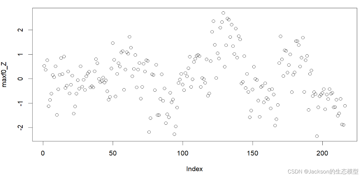
3. 2 数据标准化（Z-scores）

z分数（z-score），也叫标准分数（standard score）是一个数与平均数的差再除以标准差的过程。在统计学中，标准分数是一个观测或数据点的值高于被观测值或测量值的平均值的标准偏差的符号数。

#transfer the data to z-score
maxf0_Z<-scale(MaxF0$maxf0st,center=TRUE,scale=TRUE)
plot(maxf0_Z)

在这里插入图片描述

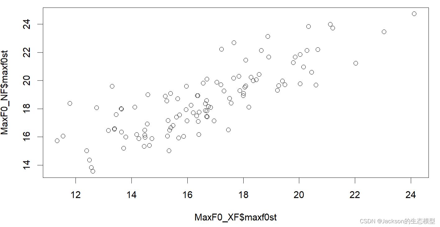
3.3 绘制数据相关性

# plot correlations
MaxF0_XF<-subset(MaxF0,MaxF0$Focus=="XF")
MaxF0_NF<-subset(MaxF0,MaxF0$Focus=="NF")plot(MaxF0_XF$maxf0st,MaxF0_NF$maxf0st)

在这里插入图片描述

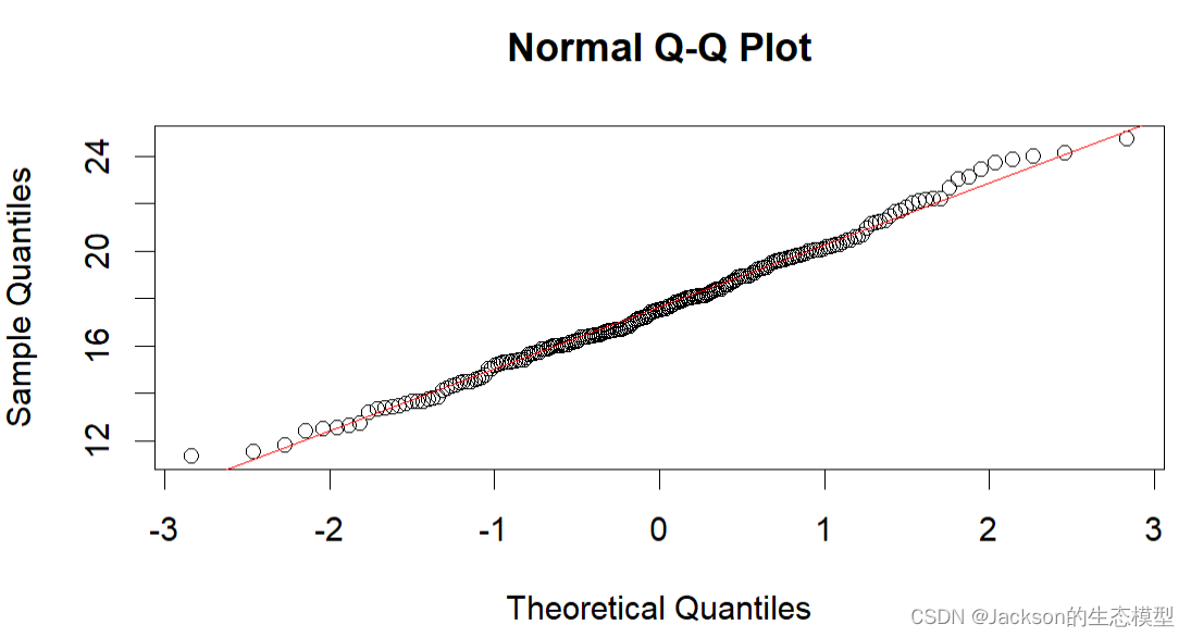
QQ图可以反映数据是否符合正态分布：

# Check whehther the data is with a normal distribution
hist(MaxF0$maxf0st)
qqnorm(MaxF0$maxf0st)
qqline(MaxF0$maxf0st,col="red")

在这里插入图片描述

绘制一行三列的直方图：

library(dplyr)
par(mfrow=c(1,3))
hist(MaxF0[MaxF0$Boundary=="Word",]$maxf0st,col="light blue",xlab="MaxF0 (st)")
hist(MaxF0[MaxF0$Boundary=="Clause",]$maxf0st,col="green",xlab="MaxF0 (st)")
hist(MaxF0[MaxF0$Boundary=="Sentence",]$maxf0st,col="grey",xlab="MaxF0 (st)")
par(mfrow=c(1,1))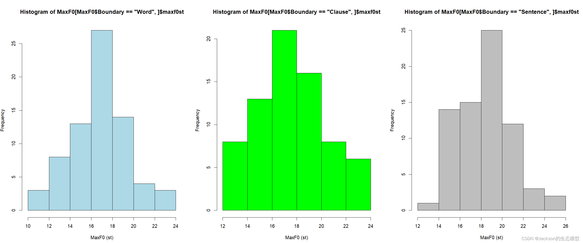

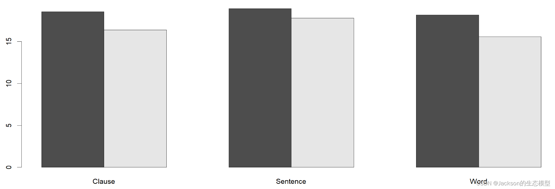
在这里插入图片描述

不同组的数据对比：

#Show the mean across groups with bars
maxf0Mean<-with(MaxF0,tapply(maxf0st, list(Focus, Boundary),mean))
maxf0Meanbarplot(maxf0Mean,beside=T)

在这里插入图片描述

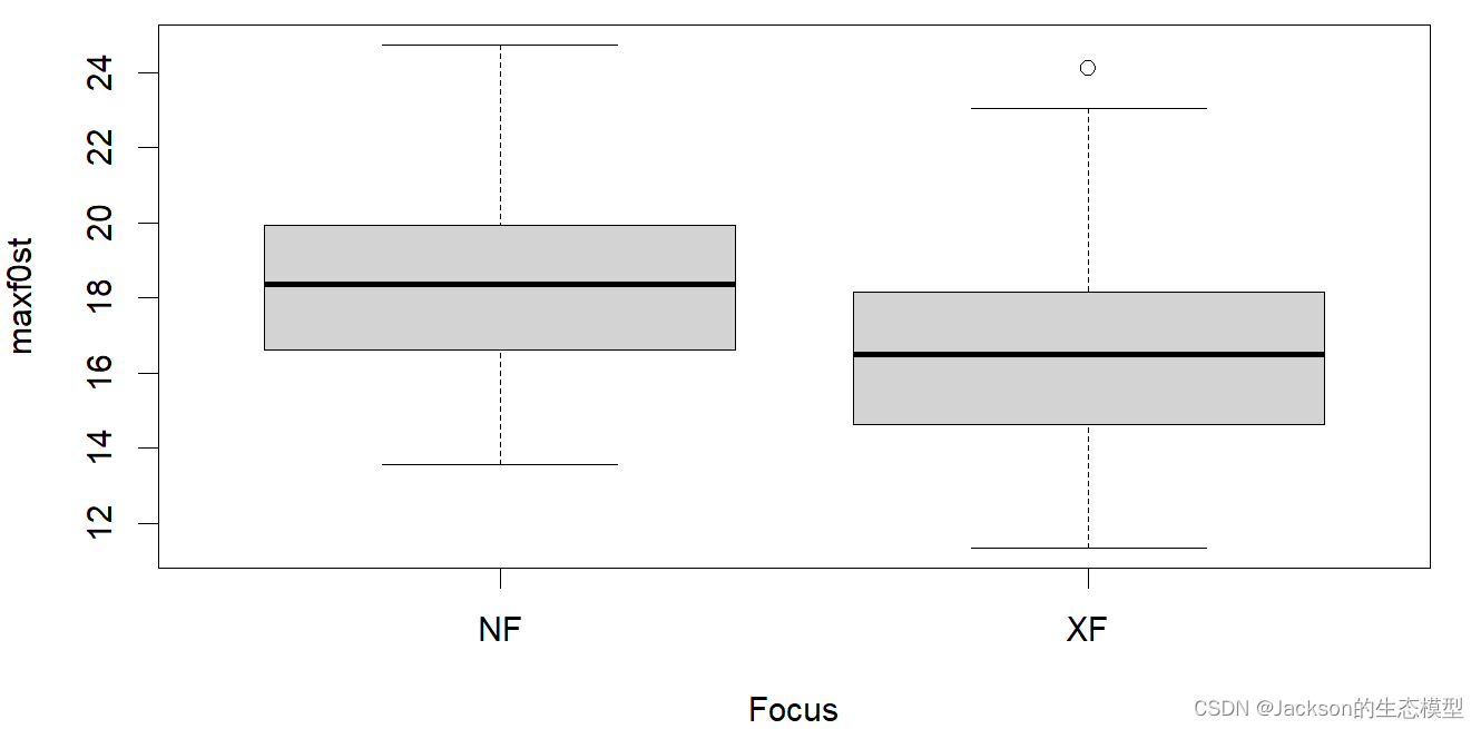
用箱线图检查各组之间是否有差异：

# check whether there is any difference bewteen groups with a boxplot
maxf0_boxplot<-boxplot(maxf0st~Focus,data=MaxF0)
maxf0_boxplot<-boxplot(maxf0st~Focus*Boundary,data=MaxF0)

在这里插入图片描述

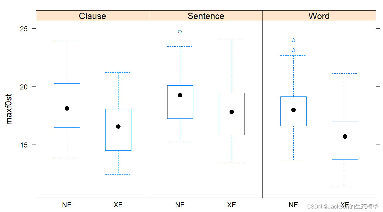
图像美化：

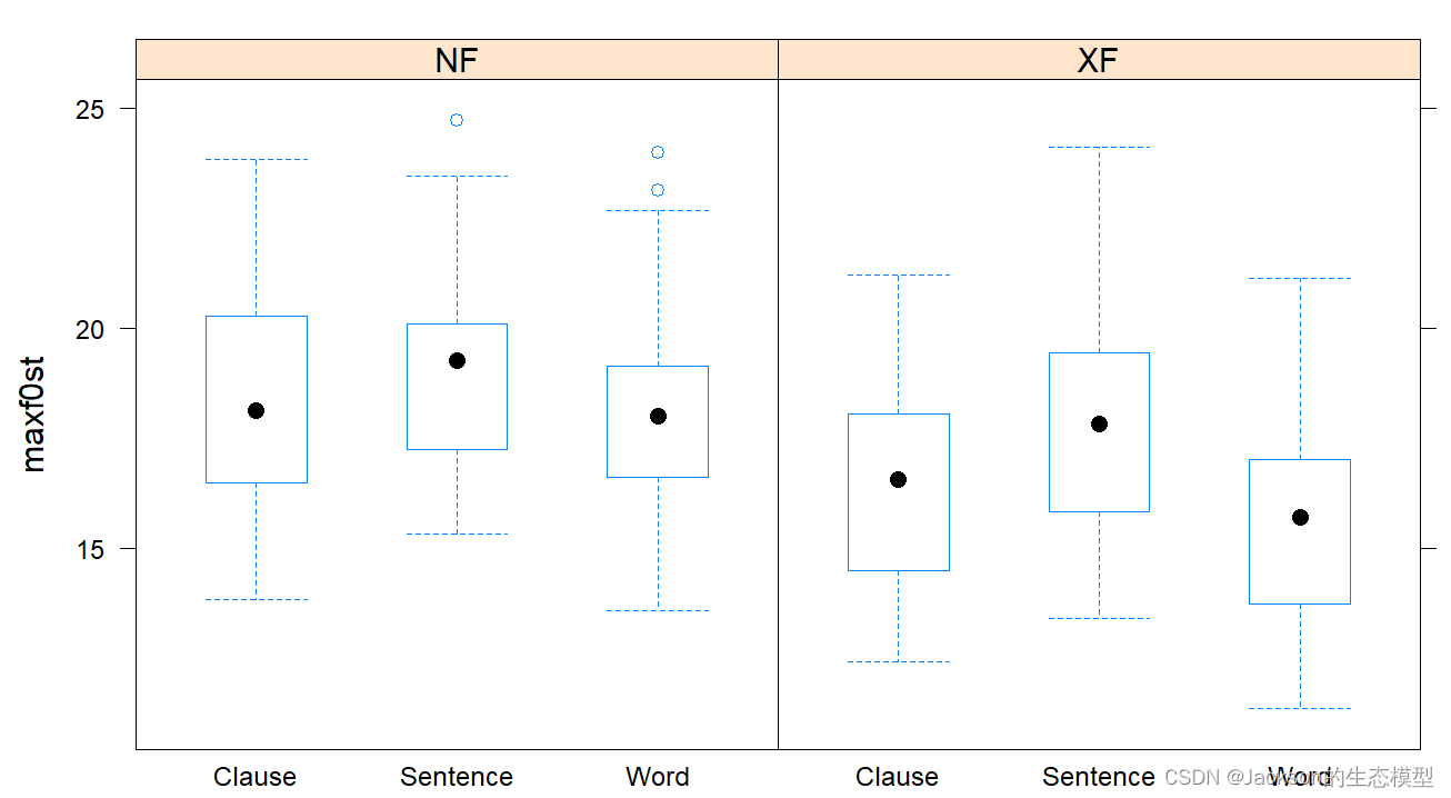
# Use lattice to display boxplots of multiple variables
library(lattice)
bwplot(maxf0st~Focus|Boundary,data=MaxF0)
bwplot(maxf0st~Boundary|Focus,data=MaxF0)

在这里插入图片描述

4、ggplot绘图

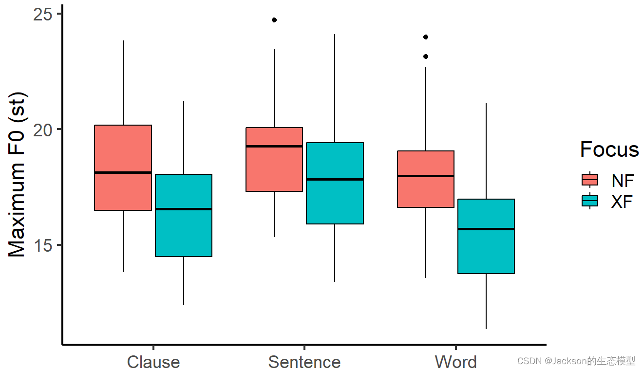
4.1 geom_boxplot

# boxplot
f0_box<-ggplot(data = MaxF0, aes(x = Boundary, y = maxf0st,color=Focus))
f0_box1<-f0_box+geom_boxplot(aes(fill = Focus),color="black",position=position_dodge(0.8))
f0_box2<-f0_box1+labs(x =element_blank(), y = "Maximum F0 (st)")
f0_box3<-f0_box2+theme_classic(base_size = 18)
f0_box3

在这里插入图片描述

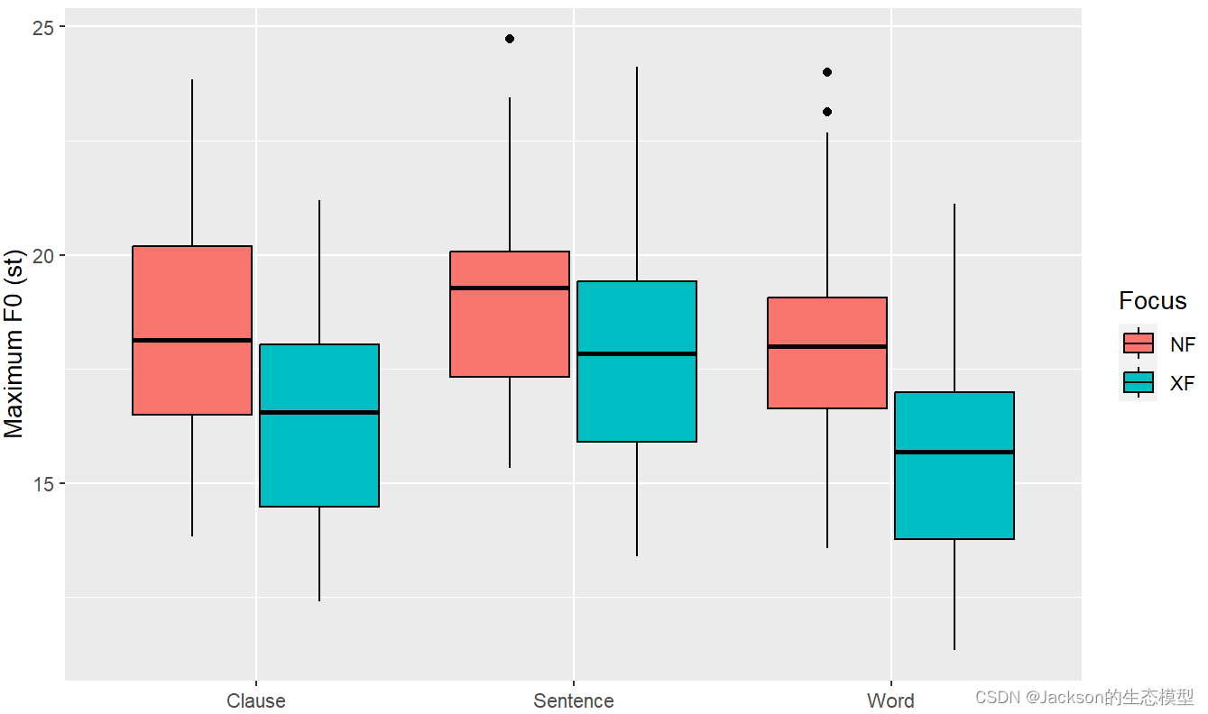
f0_box4<-f0_box2+theme_update()
f0_box4

在这里插入图片描述

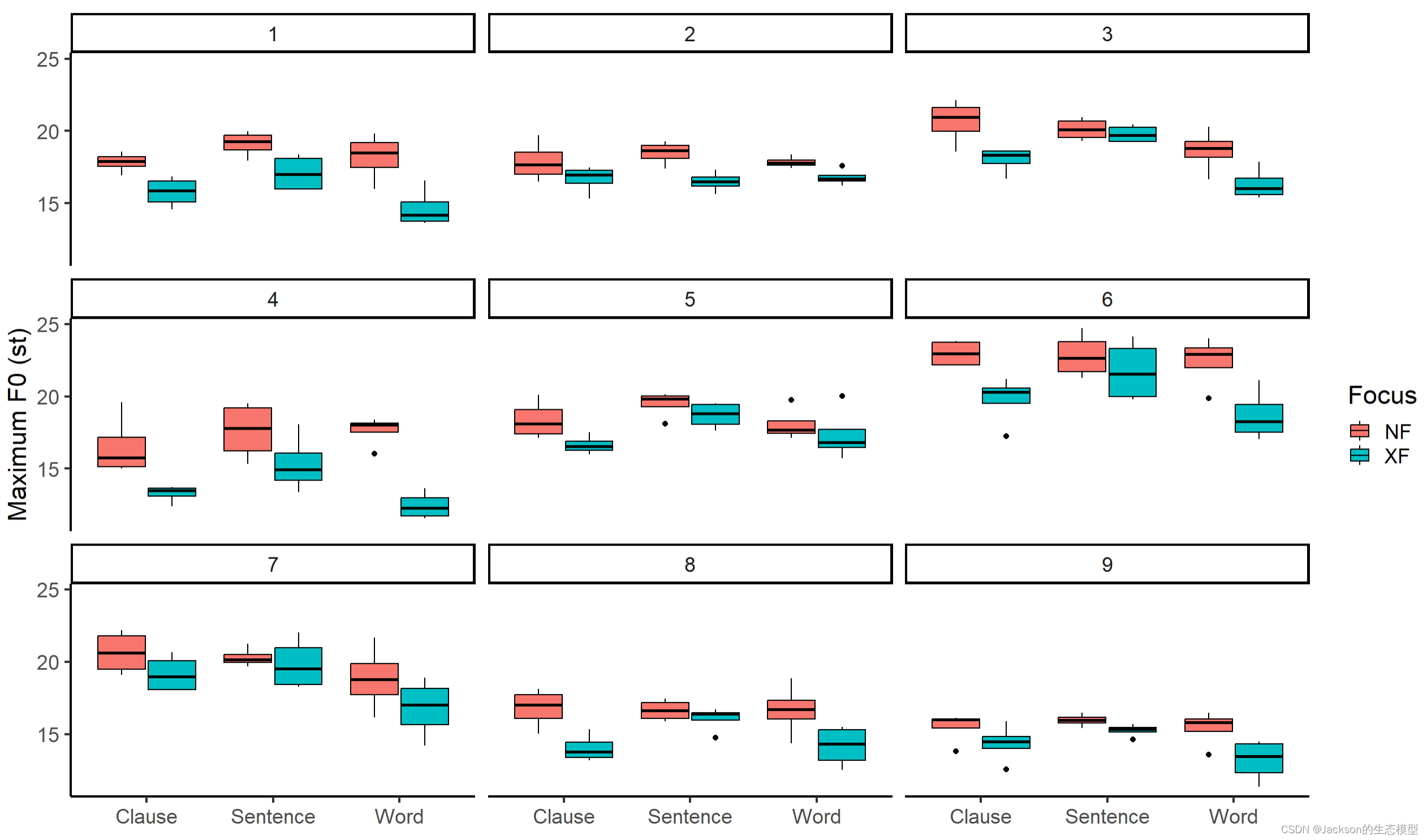
使用facet_wrap（）函数将数据展开：

#Split a plot into a matrix of panels
f0_box4<-f0_box3+facet_wrap(~Speaker,nrow=3)
f0_box4

在这里插入图片描述

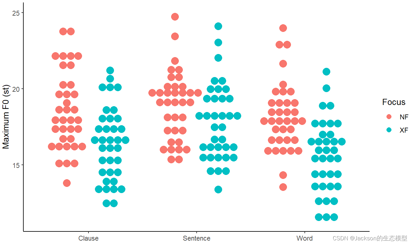
4.2 geom_dotplot()

绘制散点图：

# dotplot
f0_point<-ggplot(data = MaxF0, aes(x = Boundary, y = maxf0st,color=Focus))
f0_point1<-f0_point+geom_dotplot(aes(color = Focus,fill=Focus),binaxis = "y", stackdir = "center",position=position_dodge(0.8),dotsize =1,binwidth = 0.5)+labs(x =element_blank(), y = "Maximum F0 (st)")+theme_classic()
f0_point1
mean(MaxF0$maxf0st)#17.6

在这里插入图片描述

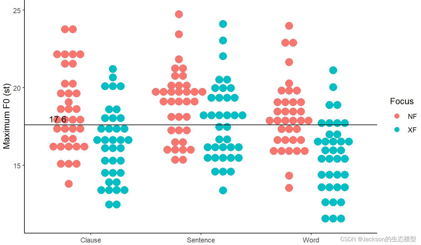
为以上图像添加平均值基线：

MaxF0$Speaker=as.factor(MaxF0$Speaker)f0_point2<-f0_point1+geom_hline(aes(yintercept=17.6))+annotate("text", x=0.7, y=18, label="17.6",size=4) 
f0_point3<-f0_point2
f0_point3

在这里插入图片描述

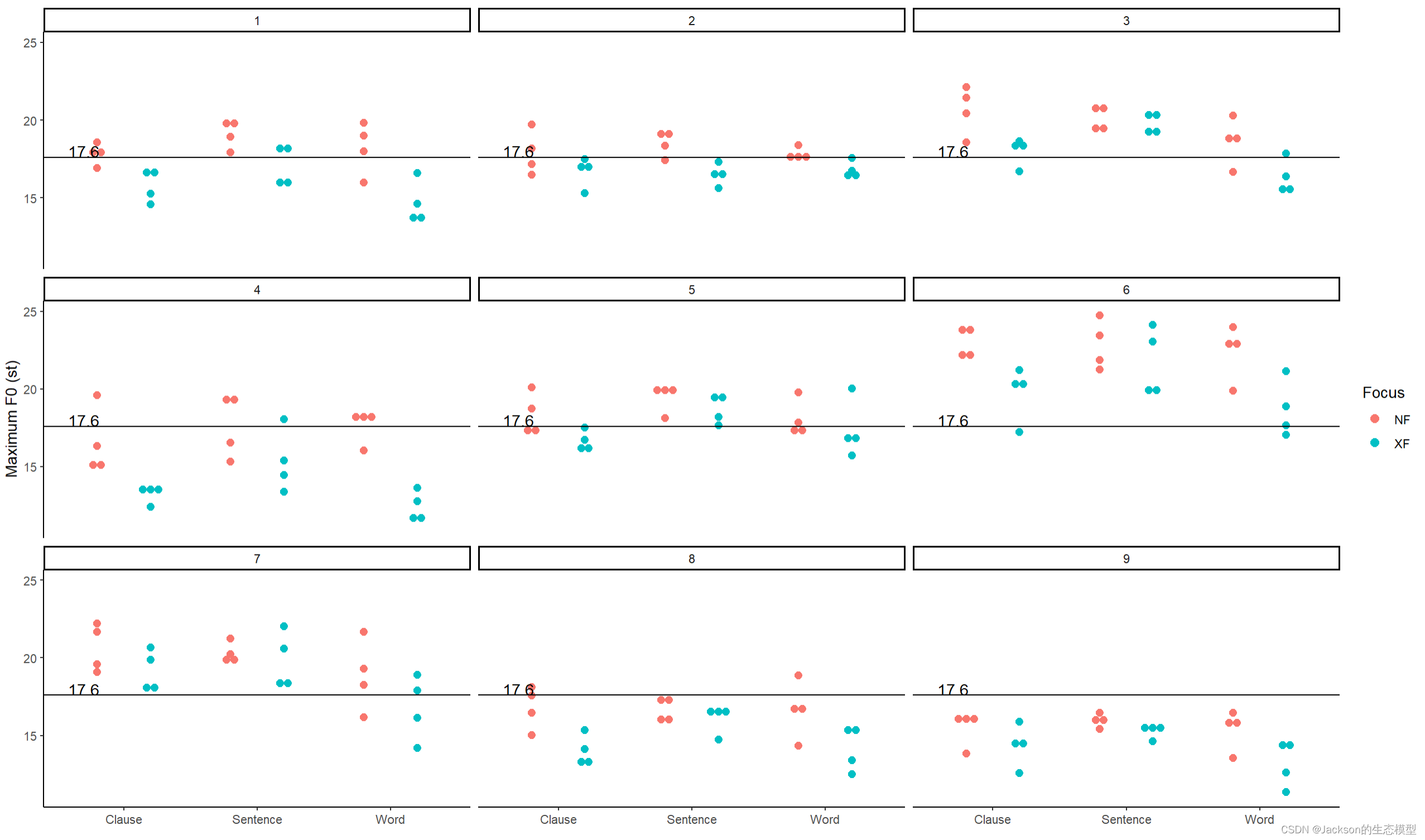
为所有分组数据添加均值基线：

f0_point4<-f0_point3+facet_wrap(~Speaker,nrow=3)
f0_point4

在这里插入图片描述

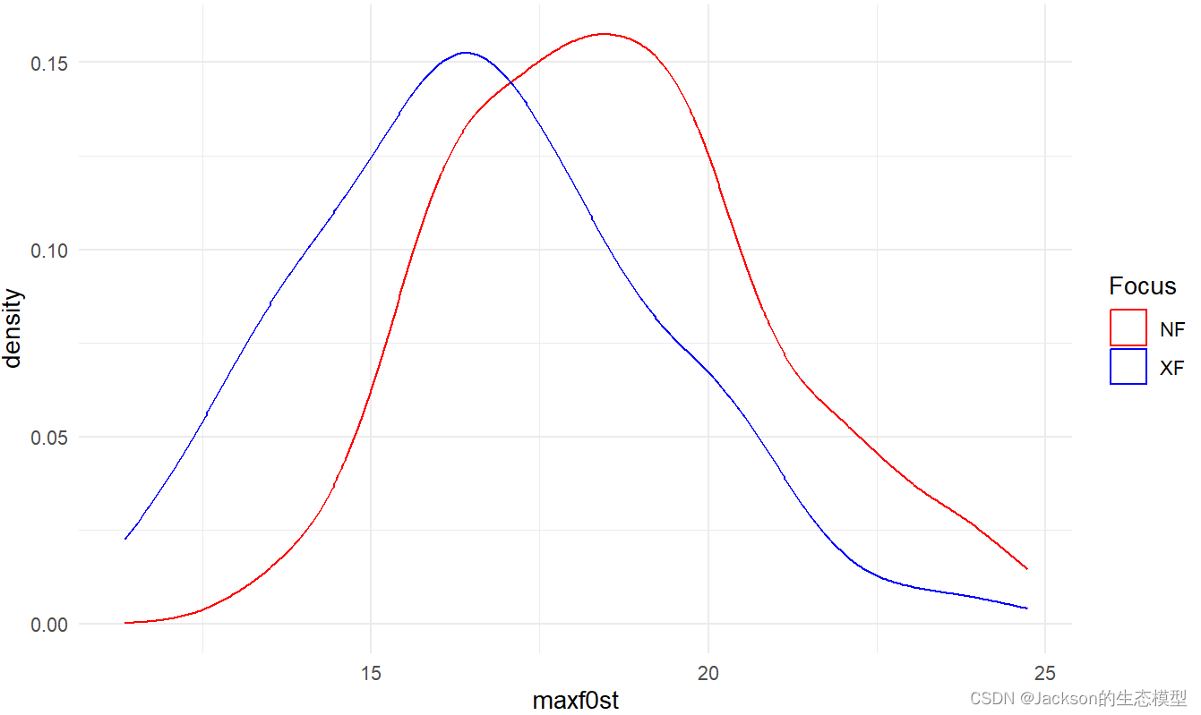
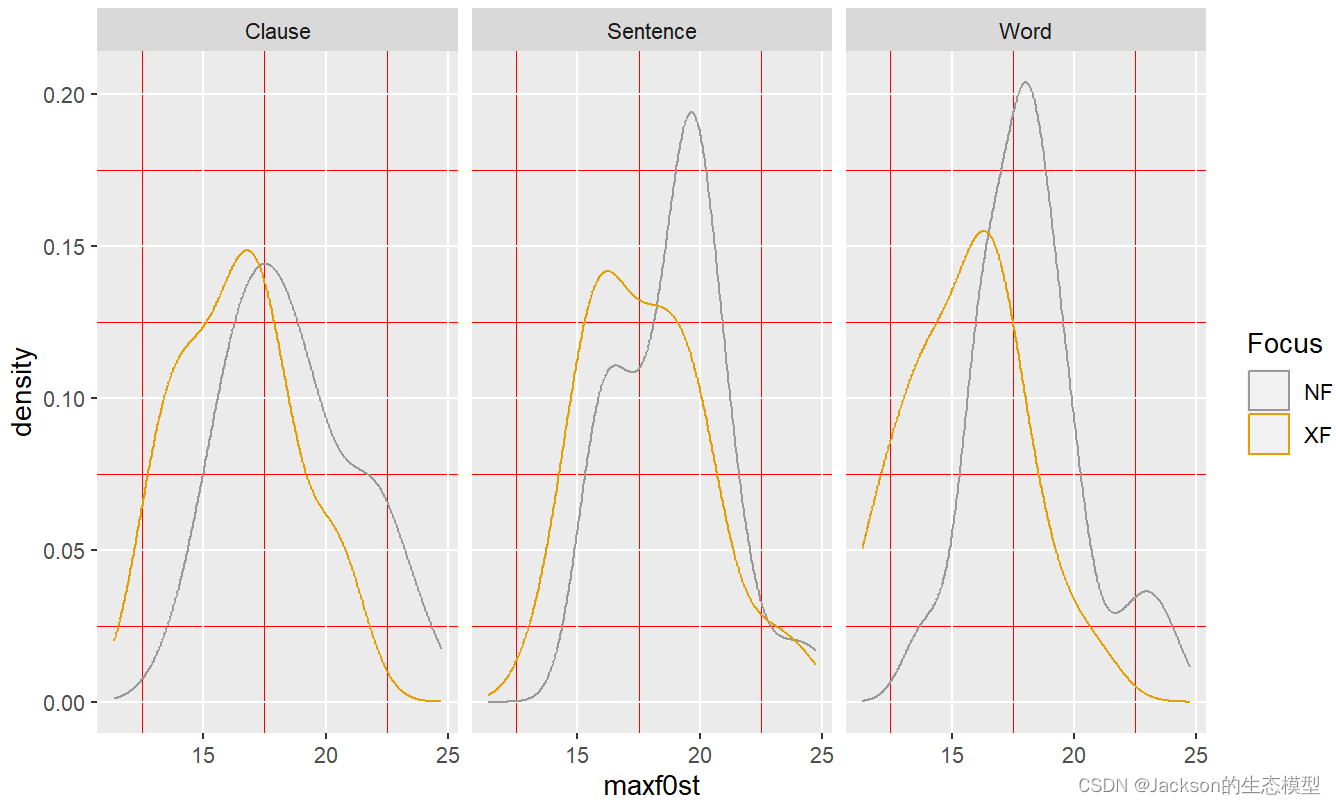
4.3 geom_density

#Density plot
f0density<-ggplot(data = MaxF0, aes(x = maxf0st,color=Focus))
f0density1<-f0density+geom_density()
f0density2<-f0density1+scale_color_manual(values=c("red", "blue"))
f0density3<-f0density2+theme_minimal()
f0density3

在这里插入图片描述

#Split a plot into a matrix of panels
f0densityf<-ggplot(data = MaxF0, aes(x = maxf0st,color=Focus))
f0densityf1<-f0densityf+geom_density()+facet_wrap(~Boundary,nrow=1)
f0densityf2<-f0densityf1+scale_color_manual(values=c("#999999", "#E69F00"))
f0densityf2

在这里插入图片描述

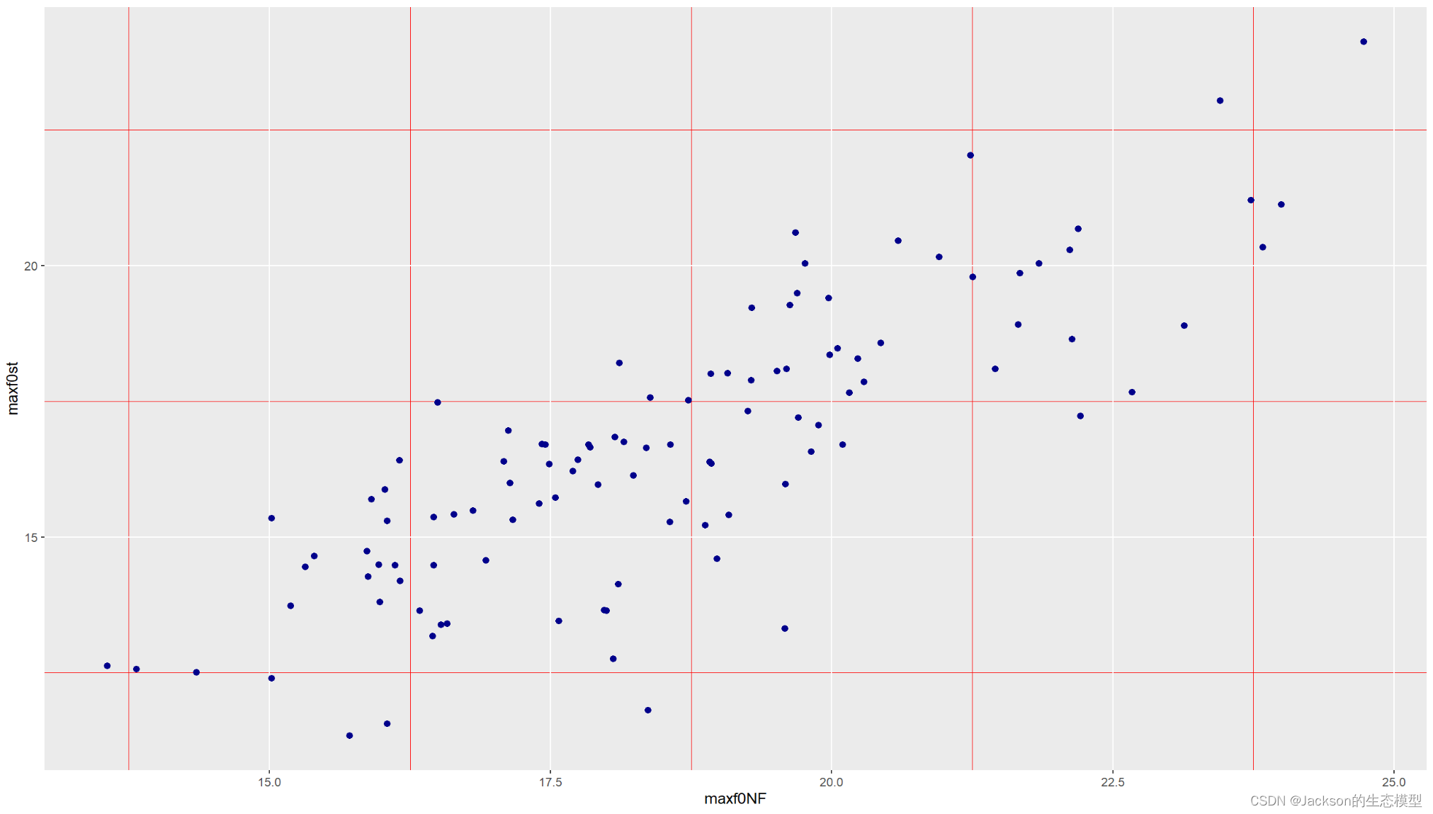
5、相关性

计算两个变量之间的相关性：

MaxF0_XF<-subset(MaxF0,MaxF0$Focus=="XF")
MaxF0_NF<-subset(MaxF0,MaxF0$Focus=="NF")cor(MaxF0_XF$maxf0st,MaxF0_NF$maxf0st) # r=0.81

提取指定数据并合并：

NFXF<-cbind(MaxF0_XF,MaxF0_NF$maxf0st)
NFXF<-data.frame(NFXF)
View(NFXF)
NFXF2<-rename(NFXF,c("maxf0st"="maxf0XF","MaxF0_NF.maxf0st"="maxf0NF"))# Put the new name first, then the old name
View(NFXF2)corNX<-ggplot(NFXF2, aes(x=maxf0NF,y=maxf0XF,))
corNX1<-corNX+geom_point(size=2,color="dark blue")
corNX1

corNX<-ggplot(NFXF2, aes(x=maxf0NF,y=maxf0st,))
corNX1<-corNX+geom_point(size=2,color="dark blue")
corNX1

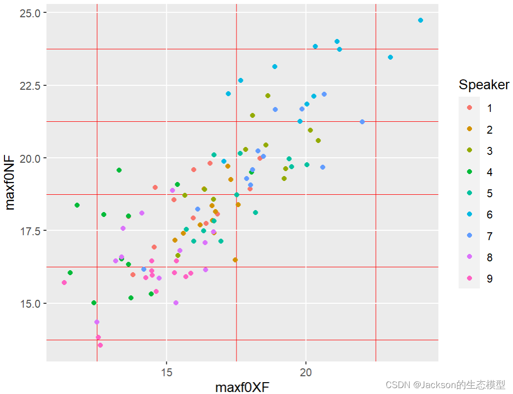
结果展示：
在这里插入图片描述

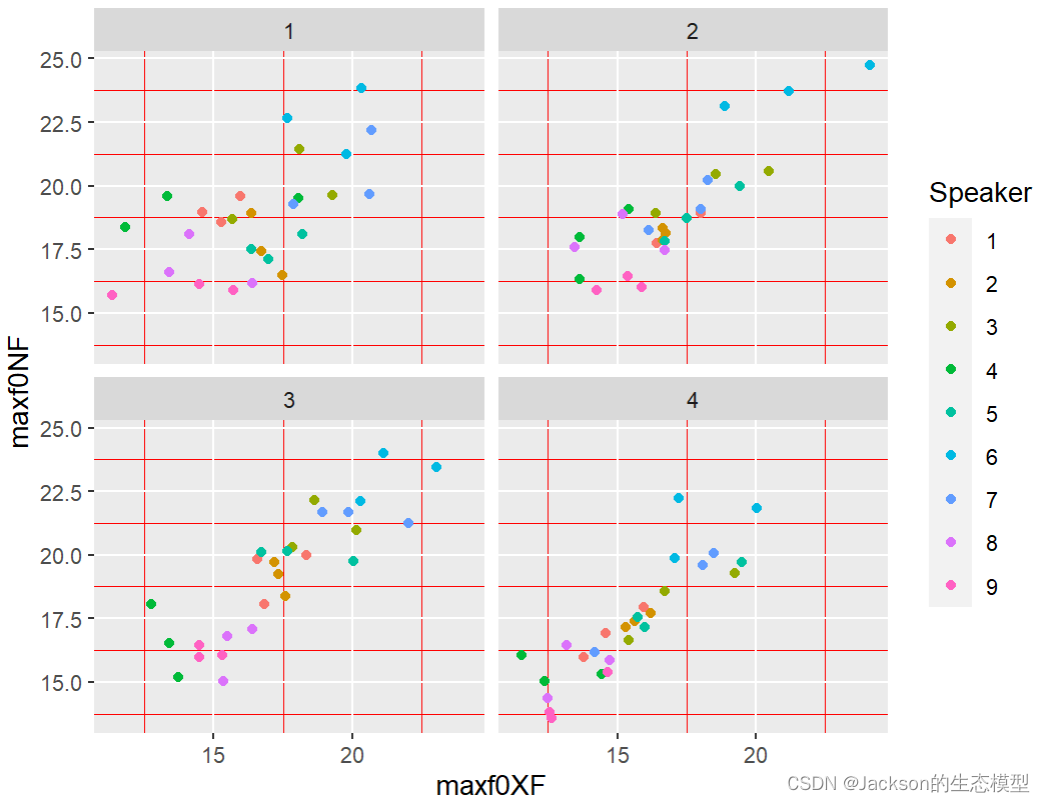
NFXF2$Speaker=as.factor(NFXF2$Speaker)corNX<-ggplot(NFXF2, aes(x=maxf0XF,y=maxf0NF,color=Speaker))
corNX1<-corNX+geom_point()
corNX1

在这里插入图片描述
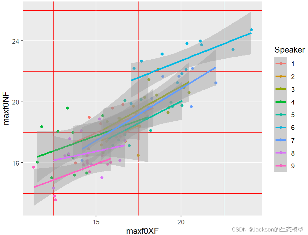
添加回归线及其置信区间：

corNXlm<-ggplot(NFXF2, aes(x=maxf0XF,y=maxf0NF))
corNXlm1<- corNXlm+geom_point()+geom_smooth(method=lm)
corNXlm1

在这里插入图片描述

corNX<-ggplot(NFXF2, aes(x=maxf0XF,y=maxf0NF,color=Speaker))
corNX1<-corNX+geom_point()+geom_smooth(method=lm)
corNX1

在这里插入图片描述

NFXF2$Speaker=as.factor(NFXF2$Speaker)
corNX<-ggplot(NFXF2, aes(x=maxf0XF,y=maxf0NF,color=Speaker))
corNX1<-corNX+geom_point()+facet_wrap(~sentence,nrow=2)
corNX1

在这里插入图片描述

6、T检验

boxplot(MaxF0$maxf0st,MaxF0$Focus)
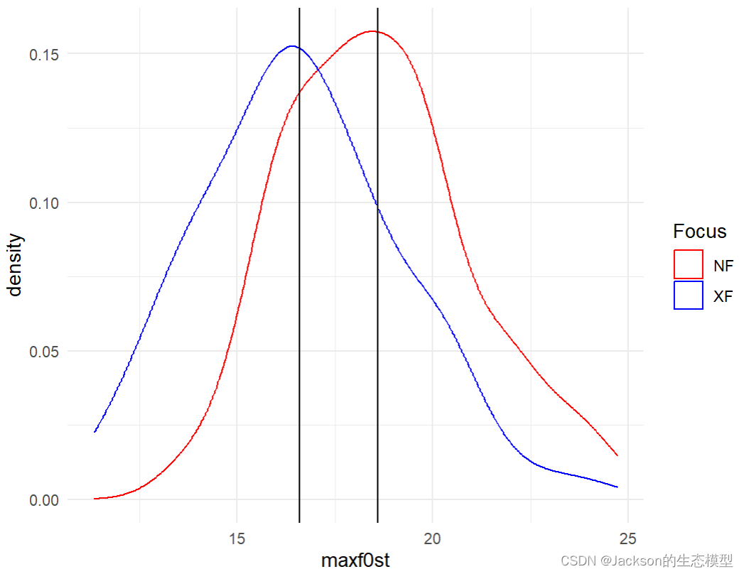
f0density<-ggplot(data = MaxF0, aes(x = maxf0st,color=Focus))
f0density1<-f0density+geom_density()
f0density2<-f0density1+scale_color_manual(values=c("red", "blue"))
f0density3<-f0density2+theme_minimal()
f0density3XF<-MaxF0[MaxF0$Focus=="XF",]$maxf0st
NF<-MaxF0[MaxF0$Focus=="NF",]$maxf0st
mean(XF) #16.6
mean(NF) #18.6f0density4<-f0density3+geom_vline(xintercept=c(16.6,18.6))
f0density4t.test(XF,NF,paired=TRUE,alternative="two.sided")

在这里插入图片描述

> t.test(XF,NF,paired=TRUE,alternative="two.sided")Paired t-testdata:  XF and NF
t = -13.607, df = 107, p-value < 2.2e-16
alternative hypothesis: true mean difference is not equal to 0
95 percent confidence interval:-2.250911 -1.678460
sample estimates:
mean difference -1.964686

7、线性回归&ANOVA

7.1 绘制主效应及其交互效应

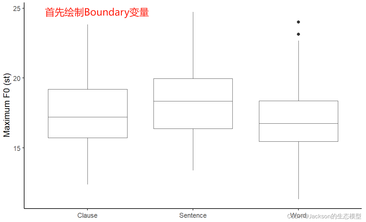
f0_boundary<-ggplot(data = MaxF0, aes(x = Boundary, y = maxf0st))
f0_boundary1<-f0_boundary+geom_boxplot(position=position_dodge(0.8),size=0.1)+labs(x =element_blank(), y = "Maximum F0 (st)")+theme_classic()
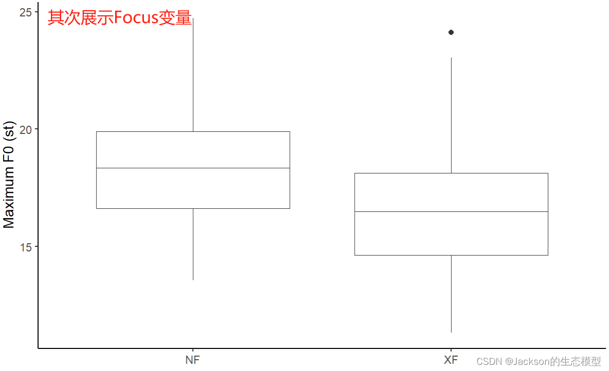
f0_boundary1f0_focus<-ggplot(data = MaxF0, aes(x = Focus, y = maxf0st))
f0_focus1<-f0_focus+geom_boxplot(position=position_dodge(0.8),size=0.1)+labs(x =element_blank(), y = "Maximum F0 (st)")+theme_classic()
f0_focus1f0_interaction<-ggplot(data = MaxF0, aes(x = Boundary, y = maxf0st))
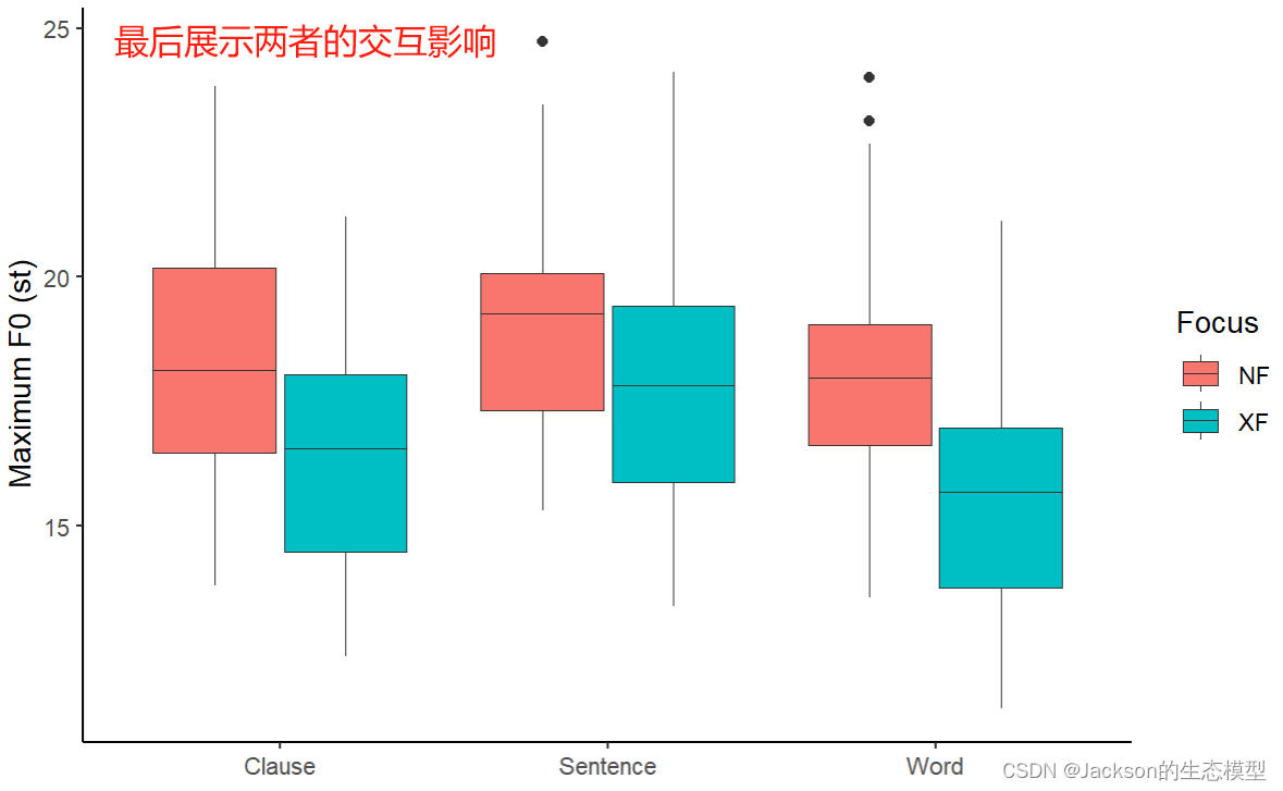
f0_interaction1<-f0_interaction+geom_boxplot(aes(fill = Focus),position=position_dodge(0.8),size=0.1)
f0_interaction2<-f0_interaction1+ scale_color_brewer(palette="Dark2")+labs(x =element_blank(), y = "Maximum F0 (st)")+theme_classic()
f0_interaction2

在这里插入图片描述

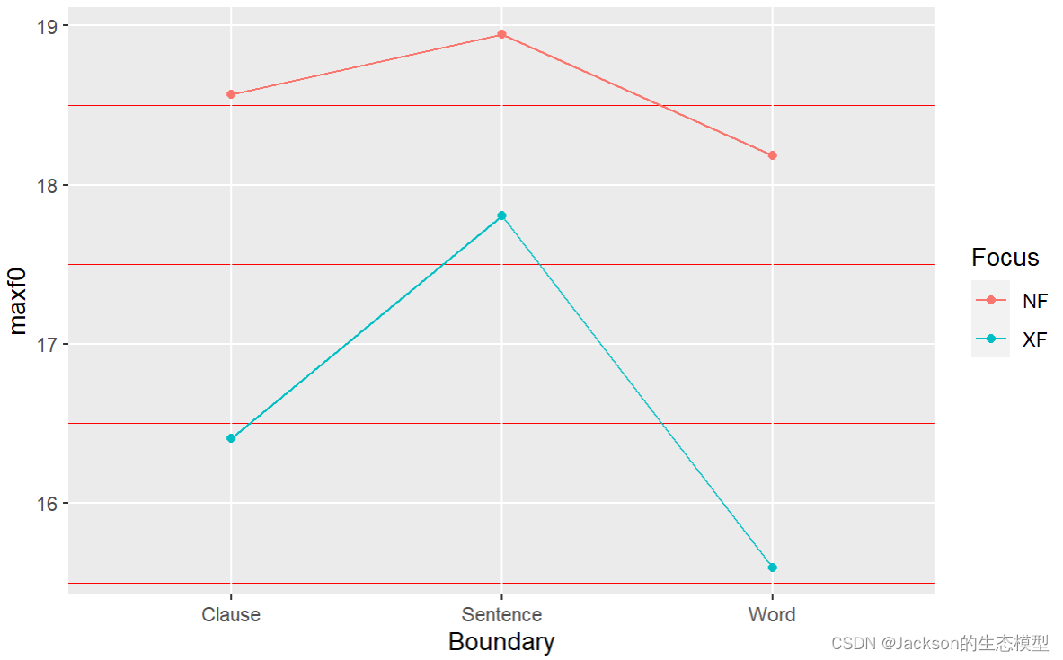
也可以使用折线图进行展示，这里使用了之前提到的==aggregate()==函数：

# Use lines to display the interaction
maxf0Mean2=aggregate(MaxF0$maxf0st,list(MaxF0$Focus,MaxF0$Boundary),mean)
maxf0Mean2
maxf0Mean2<-data.frame(maxf0Mean2)names(maxf0Mean2)=c("Focus","Boundary","maxf0") # add column neames
View(maxf0Mean2)
str(maxf0Mean2)maxf0line<-ggplot(maxf0Mean2,aes(x=Boundary,y=maxf0,group=Focus,color=Focus))
maxf0line1<-maxf0line+geom_line()+geom_point()
maxf0line1

在这里插入图片描述

7.2 ANOVA

ANOVA的本质就是线性模型（lm），因此他要求数据之间要具有独立性、正态性和同方差性等。之前已经对数据的正态性进行了检验，且已满足，但是这里的独立性可能无法满足，因此之后将涉及到线性混合效应模型。

####ANOVA
f0aov<-aov(maxf0st~Focus*Boundary,data=MaxF0)
summary(f0aov)

结果展示：

> summary(f0aov)Df Sum Sq Mean Sq F value   Pr(>F)    
Focus            1  208.4  208.44  36.380 7.23e-09 ***
Boundary         2   80.5   40.26   7.027  0.00111 ** 
Focus:Boundary   2   20.0   10.00   1.745  0.17724    
Residuals      210 1203.2    5.73                     
---
Signif. codes:  0 ‘***’ 0.001 ‘**’ 0.01 ‘*’ 0.05 ‘.’ 0.1 ‘ ’ 1

可以看出两个变量（Focus和Boundary）之间并没有交互作用。

7.3 线性模型

NXlm<-lm(maxf0XF~maxf0NF,data=NFXF2)
coef(NXlm)#y=0.08+0.88x
print(NXlm)
plot(NFXF2$maxf0NF,NFXF2$maxf0XF)
abline(NXlm,col="red")

结果展示：

> coef(NXlm)#y=0.08+0.88x
(Intercept)     maxf0NF 0.08129193  0.88980567 
> print(NXlm)Call:
lm(formula = maxf0XF ~ maxf0NF, data = NFXF2)Coefficients:
(Intercept)      maxf0NF  0.08129      0.88981

Linear-model

### Linear-model
# The lm is to test whether Focus and Boundary have any effect on maxf0st
f0lm0<-lm(maxf0st~Focus*Boundary,data=MaxF0)
summary(f0lm0)coef(f0lm0) #coefficient
confint(f0lm0) #confident intervalanova(f0lm0)# It then gives the results in the ANOVA style

结果展示：

> summary(f0lm0)Call:
lm(formula = maxf0st ~ Focus * Boundary, data = MaxF0)Residuals:Min     1Q Median     3Q    Max 
-4.751 -1.850 -0.006  1.466  6.316 Coefficients:Estimate Std. Error t value Pr(>|t|)    
(Intercept)               18.5696     0.3989  46.547  < 2e-16 ***
FocusXF                   -2.1621     0.5642  -3.832 0.000168 ***
BoundarySentence           0.3766     0.5642   0.667 0.505231    
BoundaryWord              -0.3845     0.5642  -0.681 0.496353    
FocusXF:BoundarySentence   1.0214     0.7979   1.280 0.201890    
FocusXF:BoundaryWord      -0.4292     0.7979  -0.538 0.591204    
---
Signif. codes:  0 ‘***’ 0.001 ‘**’ 0.01 ‘*’ 0.05 ‘.’ 0.1 ‘ ’ 1Residual standard error: 2.394 on 210 degrees of freedom
Multiple R-squared:  0.2043,	Adjusted R-squared:  0.1854 
F-statistic: 10.78 on 5 and 210 DF,  p-value: 3.039e-09

FocusXF处的结果表明，FocusXF与FocusNF相比，比起均值低2.1621，且P显著，表明二者存在显著差异。
BoundarySentence和BoundaryWord 的结果均是和BoundaryClause相比，且结果不显著，表明三者并无显著差异。
此外，值得注意的是，t value=Estimate/Std. Error，且|t value|>1.96，则近似于P<0.05。

T value here tells us whether the coefficients are significantly different from zero. When t>1.96, it indicates that p<0.05.
这里使用别人的图进行解释：

> anova(f0lm0)
Analysis of Variance TableResponse: maxf0stDf  Sum Sq Mean Sq F value    Pr(>F)    
Focus            1  208.44 208.439 36.3799 7.228e-09 ***
Boundary         2   80.53  40.263  7.0273  0.001111 ** 
Focus:Boundary   2   19.99   9.996  1.7446  0.177239    
Residuals      210 1203.20   5.730                      
---
Signif. codes:  0 ‘***’ 0.001 ‘**’ 0.01 ‘*’ 0.05 ‘.’ 0.1 ‘ ’ 1

其中Residuals为残差（真实值与估计值之差），表示线性模型中无法解释的变化。
此处的anova()的结果与上面7.2节中使用的 f0aov<-aov(maxf0st~Focus*Boundary,data=MaxF0) 函数的结果基本一致。因此使用两种方法进行ANOVA检验都是可以的。

由于线性模型中的数据无法满足独立性的要求，因此存在很多的不确定因素，因此我们可以将其中的一些变量作为随机变量，如speaker或者sentence，如下所示：

# by-subject vs. by-item analysis
f0aov_er<-aov(maxf0st~Focus*Boundary+Error(Speaker),data=MaxF0)
summary(f0aov_er)f0aov_er2<-aov(maxf0st~Focus*Boundary+Error(sentence),data=MaxF0)
summary(f0aov_er2)

结果展示：

> summary(f0aov_er)Error: SpeakerDf Sum Sq Mean Sq F value Pr(>F)
Residuals  1  19.45   19.45               Error: WithinDf Sum Sq Mean Sq F value   Pr(>F)    
Focus            1  208.4  208.44  36.802 6.05e-09 ***
Boundary         2   80.5   40.26   7.109  0.00103 ** 
Focus:Boundary   2   20.0   10.00   1.765  0.17376    
Residuals      209 1183.7    5.66                     
---
Signif. codes:  
0 ‘***’ 0.001 ‘**’ 0.01 ‘*’ 0.05 ‘.’ 0.1 ‘ ’ 1

> summary(f0aov_er2)Error: sentenceDf Sum Sq Mean Sq F value Pr(>F)
Residuals  1  30.71   30.71               Error: WithinDf Sum Sq Mean Sq F value   Pr(>F)    
Focus            1  208.4  208.44  37.155 5.19e-09 ***
Boundary         2   80.5   40.26   7.177 0.000967 ***
Focus:Boundary   2   20.0   10.00   1.782 0.170889    
Residuals      209 1172.5    5.61                     
---
Signif. codes:  
0 ‘***’ 0.001 ‘**’ 0.01 ‘*’ 0.05 ‘.’ 0.1 ‘ ’ 1

通过残差Residuals表明，通过增加不同的随机变量，可以降低模型的不确定性，然而降低的效果确实有限。因此为了生成误差更小的模型，我们需要构建线性混合效应模型。

8、线性混合效应模型（LMM）

在这里插入图片描述

线性混合效应模型包括了两个部分，即固定效应（fixed effects）和随机效应（random effects），而随机效应部分又分为随机截距和随机斜率。我们常使用llme4包中的lmer()函数构建LMM。我们需要重点关注随机效应部分，表示方法为： (1|Speaker)：speaker作为固定截距；(1+Focus|Speaker)： speaker条件下，Focus为随机斜率且随机截距；(0+Focus|Speaker) ：speaker条件下，Focus为随机斜率且固定截距。

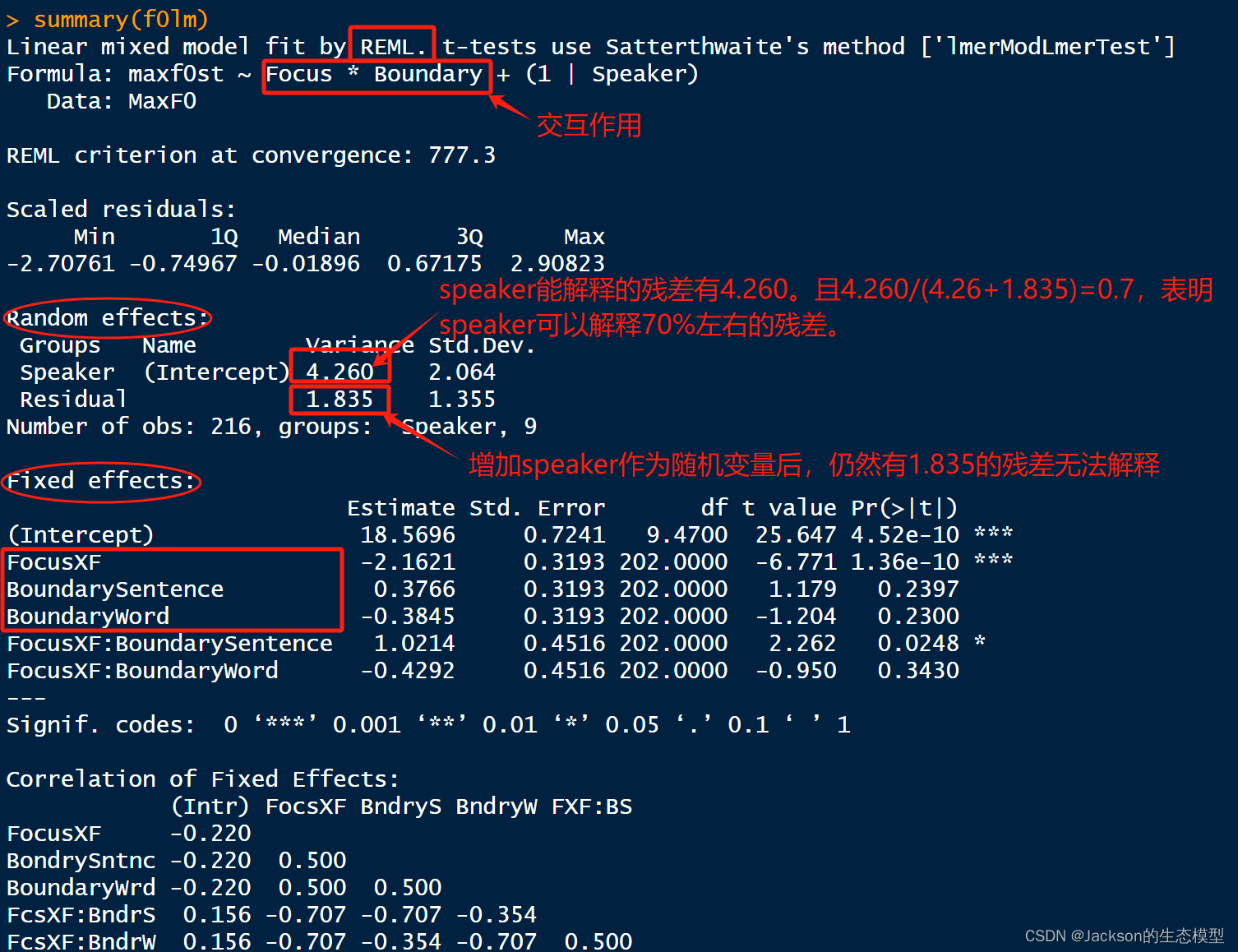
变量间存在交互作用：

#Fixed effect: Focus and Boundary, Random effect(intercept): Speaker
f0lm<-lmer(maxf0st~Focus*Boundary+(1|Speaker),data=MaxF0)
summary(f0lm)

在这里插入图片描述

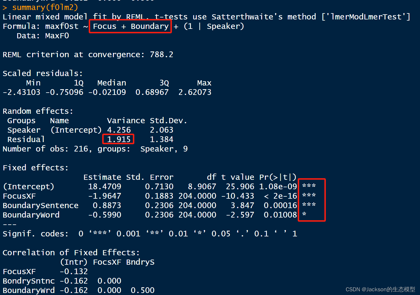
变量间不存在交互作用：

f0lm2<-lmer(maxf0st~Focus+Boundary+(1|Speaker),data=MaxF0)
summary(f0lm2)

在这里插入图片描述
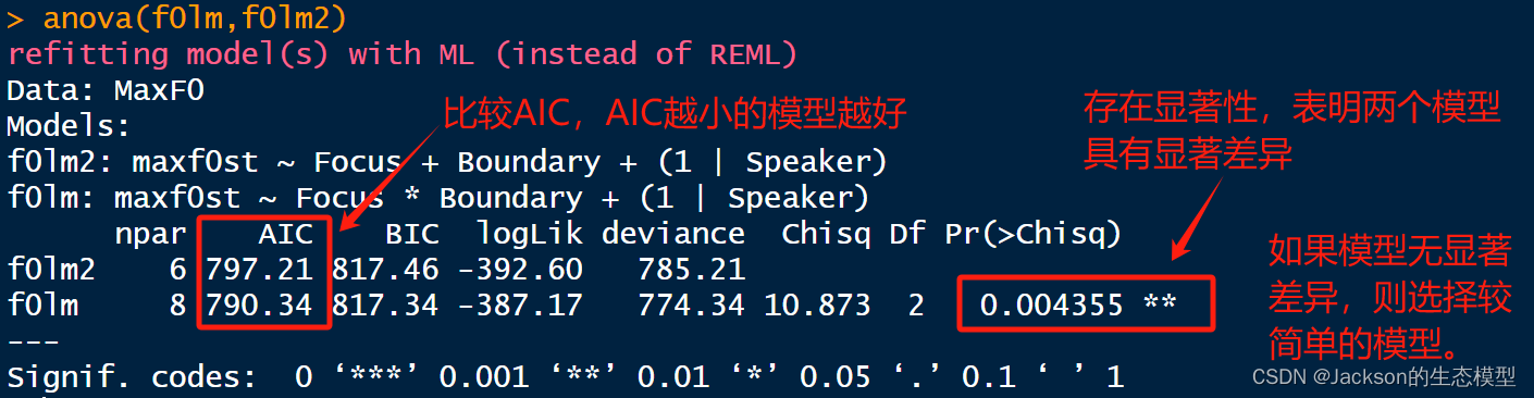
以上两个模型进行对比：

#model comparsion
anova(f0lm,f0lm2)

在这里插入图片描述

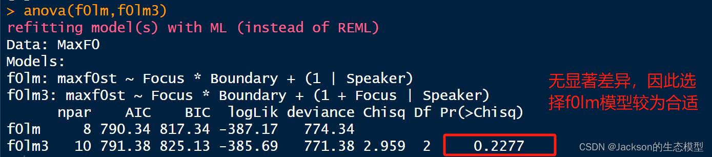
构建随机斜率模型：

#random intercept on Speaker, and random slop of Focus on Speaker
f0lm3<-lmer(maxf0st~Focus*Boundary+(1+Focus|Speaker),data=MaxF0)
summary(f0lm3)
coef(f0lm3)anova(f0lm,f0lm3)