准备数据
import pandas as pd
import numpy as np
import matplotlib.pyplot as plt
from sklearn.preprocessing import StandardScaler
from sklearn.preprocessing import OneHotEncoder
from sklearn.preprocessing import PolynomialFeatures
from sklearn.compose import ColumnTransformer
from sklearn.pipeline import Pipeline
import warnings
warnings.filterwarnings('ignore')
%matplotlib inline
%config InlineBackend.figure_format = 'retina'
# 读取数据
train = pd.read_csv("train.csv")
# print(train.head())
# 列出需要标准化的数值型特征和需要独热编码的类别型特征
numeric_features = ['age', 'duration', 'campaign', 'pdays', 'previous', 'emp_var_rate', 'cons_price_index', 'cons_conf_index', 'lending_rate3m', 'nr_employed']
categorical_features = ['job', 'marital', 'education', 'default', 'housing', 'loan', 'contact', 'month', 'day_of_week', 'poutcome']
# 定义ColumnTransformer
preprocessor = ColumnTransformer(transformers=[('poly', PolynomialFeatures(degree=3, include_bias=False), numeric_features),  # 标准化数值型特征('cat', OneHotEncoder(), categorical_features)  # 独热编码类别型特征])
# 定义包含数据处理和特征工程的Pipeline
preprocessing_pipeline = Pipeline([('preprocessor', preprocessor)  # 数据处理和特征工程
])
# 在训练集上拟合数据处理和特征工程的Pipeline
X_transformed = preprocessing_pipeline.fit_transform(train)
y = train["subscribe"].apply(lambda x: 1 if x == "yes" else 0)
模型训练和结果
使用逻辑回归/决策树/随机森林算法
from sklearn.model_selection import train_test_split
from sklearn.linear_model import LogisticRegression
from sklearn.tree import DecisionTreeClassifier
from sklearn.ensemble import RandomForestClassifier
from sklearn.metrics import confusion_matrix, accuracy_score, roc_curve, auc
import seaborn as sns# 划分训练集和测试集
X_train, X_test, y_train, y_test = train_test_split(X_transformed, y, test_size=0.3, random_state=42)# 定义模型
models = {'Logistic Regression': LogisticRegression(max_iter=1000),'Decision Tree': DecisionTreeClassifier(),'Random Forest': RandomForestClassifier(n_estimators=100)
}# 字典存储结果
results = {}for model_name, model in models.items():# 训练模型model.fit(X_train, y_train)# 预测y_pred = model.predict(X_test)# 评估accuracy = accuracy_score(y_test, y_pred)cm = confusion_matrix(y_test, y_pred)# 计算ROC曲线和AUCy_prob = model.predict_proba(X_test)[:, 1]fpr, tpr, _ = roc_curve(y_test, y_prob)roc_auc = auc(fpr, tpr)results[model_name] = {'accuracy': accuracy,'confusion_matrix': cm,'fpr': fpr,'tpr': tpr,'roc_auc': roc_auc}# 输出准确率
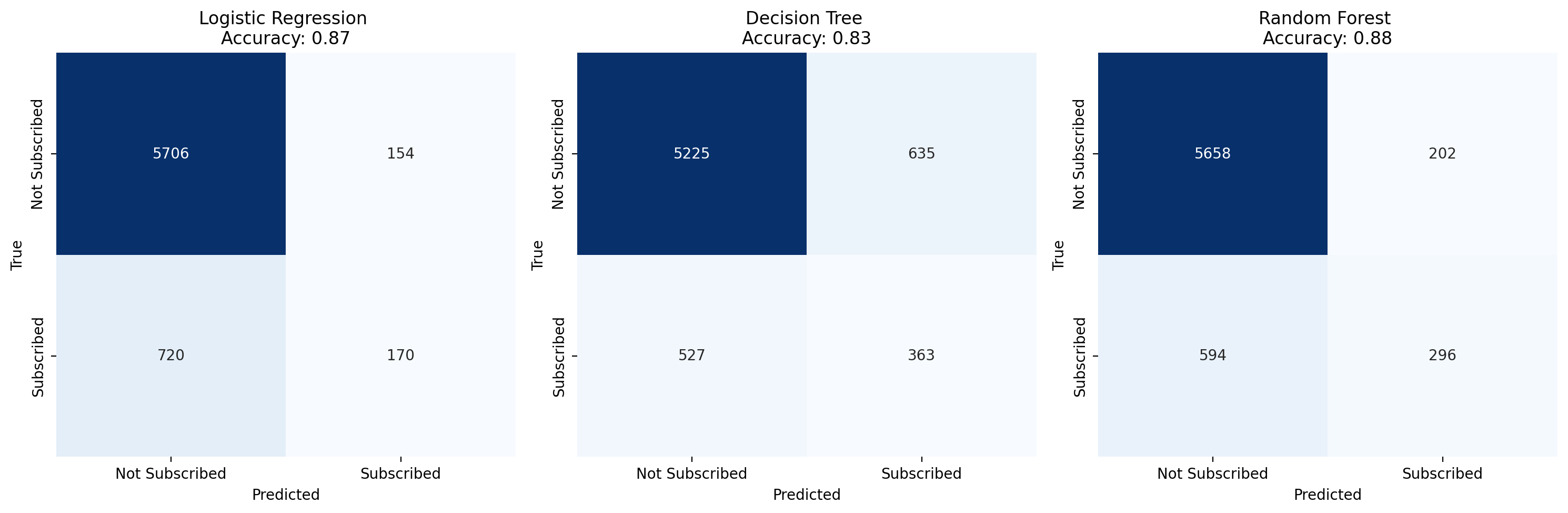
for name, metrics in results.items():print(f"{name} Accuracy: {metrics['accuracy']:.2f} - AUC: {metrics['roc_auc']:.2f}")Logistic Regression Accuracy: 0.87 - AUC: 0.82
Decision Tree Accuracy: 0.83 - AUC: 0.65
Random Forest Accuracy: 0.88 - AUC: 0.88
数据可视化
# 1. 绘制混淆矩阵
plt.figure(figsize=(15, 5)) # 创建新的图形并设置大小
for i, (model_name, metrics) in enumerate(results.items()):plt.subplot(1, 3, i + 1) # 将混淆矩阵放在1行3列的位置sns.heatmap(metrics['confusion_matrix'], annot=True, fmt='d', cmap='Blues', xticklabels=['Not Subscribed', 'Subscribed'], yticklabels=['Not Subscribed', 'Subscribed'], cbar=False)plt.title(f'{model_name} \nAccuracy: {metrics["accuracy"]:.2f}')plt.xlabel('Predicted')plt.ylabel('True')plt.tight_layout()
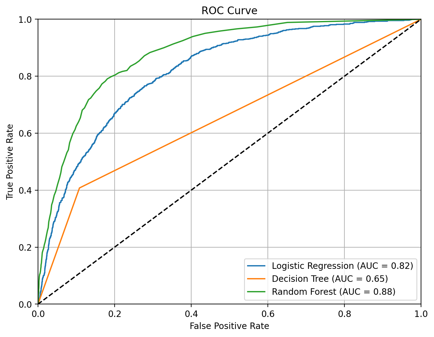
plt.show()# 2. 绘制ROC曲线
plt.figure(figsize=(8, 6)) # 创建新的图形并设置大小
for model_name, metrics in results.items():plt.plot(metrics['fpr'], metrics['tpr'], label=f'{model_name} (AUC = {metrics["roc_auc"]:.2f})')plt.plot([0, 1], [0, 1], 'k--')
plt.axis([0, 1, 0, 1])
plt.xlabel('False Positive Rate')
plt.ylabel('True Positive Rate')
plt.title('ROC Curve')
plt.legend()
plt.grid()
plt.show()
针对随机森林使用网格搜索优化
import pandas as pd
import numpy as np
import matplotlib.pyplot as plt
from sklearn.model_selection import train_test_split, GridSearchCV
from sklearn.ensemble import RandomForestClassifier
from sklearn.metrics import confusion_matrix, classification_report, roc_curve, auc
from sklearn.pipeline import Pipeline
from sklearn.compose import ColumnTransformer
from sklearn.preprocessing import OneHotEncoder, StandardScaler, PolynomialFeatures
import seaborn as sns# 读取数据
train = pd.read_csv("train.csv")# 列出需要标准化的数值型特征和需要独热编码的类别型特征
numeric_features = ['age', 'duration', 'campaign', 'pdays', 'previous', 'emp_var_rate', 'cons_price_index', 'cons_conf_index', 'lending_rate3m', 'nr_employed']
categorical_features = ['job', 'marital', 'education', 'default', 'housing', 'loan', 'contact', 'month', 'day_of_week', 'poutcome']# 定义ColumnTransformer
preprocessor = ColumnTransformer(transformers=[('poly', PolynomialFeatures(degree=3, include_bias=False), numeric_features),('cat', OneHotEncoder(), categorical_features)])# 定义随机森林模型
rf_model = RandomForestClassifier(random_state=42)# 创建Pipeline
pipeline = Pipeline(steps=[('preprocessor', preprocessor),('classifier', rf_model)])# 分割数据集
X = train.drop('subscribe', axis=1)
y = train["subscribe"].apply(lambda x: 1 if x == "yes" else 0)
X_train, X_test, y_train, y_test = train_test_split(X, y, test_size=0.3, random_state=42)# 网格搜索寻找最佳参数
param_grid = {'classifier__n_estimators': [50, 100, 150],'classifier__max_depth': [None, 10, 20, 30],'classifier__min_samples_split': [2, 5, 10],'classifier__min_samples_leaf': [1, 2, 4]
}
grid_search = GridSearchCV(pipeline, param_grid, cv=5, scoring='f1')
grid_search.fit(X_train, y_train)# 获取最佳的模型
best_model = grid_search.best_estimator_
print(f"Best parameters: {grid_search.best_params_}")# 模型评估
y_pred = best_model.predict(X_test)
conf_matrix = confusion_matrix(y_test, y_pred)
report = classification_report(y_test, y_pred)
print(report)# 计算ROC曲线
fpr, tpr, thresholds = roc_curve(y_test, best_model.predict_proba(X_test)[:, 1])
roc_auc = auc(fpr, tpr)# 绘制混淆矩阵和ROC曲线
fig, axes = plt.subplots(1, 2, figsize=(14, 6))# 绘制混淆矩阵
sns.heatmap(conf_matrix, annot=True, fmt='d', cmap='Blues', ax=axes[0], xticklabels=['Not Subscribed', 'Subscribed'], yticklabels=['Not Subscribed', 'Subscribed'])
axes[0].set_title('Confusion Matrix')
axes[0].set_xlabel('Predicted')
axes[0].set_ylabel('Actual')# 绘制ROC曲线
axes[1].plot(fpr, tpr, color='blue', label=f'ROC curve (area = {roc_auc:.2f})')
axes[1].plot([0, 1], [0, 1], color='red', linestyle='--')
axes[1].set_xlabel('False Positive Rate')
axes[1].set_ylabel('True Positive Rate')
axes[1].set_title('Receiver Operating Characteristic')
axes[1].legend()plt.tight_layout()
plt.show()