前言：

对于之前项目中工作内容进行总结，使用Carla中的车辆进行lka算法调试，整体技术路线：

①在Carla中生成车辆，并在车辆上搭载camera，通过camera采集图像数据；

②使用图像处理lka算法，对于camera数据进行计算分析；

③对于分析的结果输出为偏移图像中心的线的距离，并以这个距离做为车辆控制方向盘的数值。

其中第一步比较简单，不做记录，从第二步，lka算法实现开始。

需要对于输入的图像进行边缘检测提取出车道线

一、边缘检测

车道线一般为黄线和白线，与车道线旁的公路的颜色有很大的差异，通过这种差异，就是车道线与公路之间颜色变化，可以找到车道线的边缘，找到这个边缘的过程为边缘检测。

1.1 使用sobel进行边缘检测

直接使用cv2中Sobel包来进行边缘检测：

测试源码如下：

def abs_sobel_thresh(image,orient='x',sobel_kernel=3,thresh=(0,255)):# generating the gray image.gray = cv2.cvtColor(image,cv2.COLOR_RGB2GRAY)# 计算x方向和y方向的梯度上强度值的图像if orient == 'x':abs_sobel = np.absolute(cv2.Sobel(gray,cv2.CV_64F,1,0,ksize=sobel_kernel))if orient == 'y':abs_sobel = np.absolute(cv2.Sobel(gray,cv2.CV_64F,0,1,ksize=sobel_kernel))# 利用归一化获得scaled_sobel = np.uint8(255*abs_sobel/np.max(abs_sobel))# 创建出一个同尺寸的数组grad_binary = np.zeros_like(scaled_sobel)grad_binary[ ( scaled_sobel >= thresh[0] ) & ( scaled_sobel <= thresh[1] ) ] = 1return grad_binary

主要功能实现在abs_sobel_thresh函数中，

首先使用cv2.cvtColor函数将原始图像转化为灰度图，

然后计算x方向和y方向上的梯度强度值上的图像，

利用归一化获得一个数组，这个数组记录了图像中所有的点的强度值，然后新建一个同样size的图像数组，将数组中强度信息在0到255之间的值设置为1。

输出x和y方向梯度的图像对比：

    ksize = 15gradx = abs_sobel_thresh(image,orient='x',sobel_kernel=ksize,thresh=(50,180))grady = abs_sobel_thresh(image,orient='y',sobel_kernel=ksize,thresh=(30,90))fig1 = plt.figure()plt.imshow(gradx,cmap="gray")fig2 = plt.figure()plt.imshow(grady,cmap="gray")plt.show()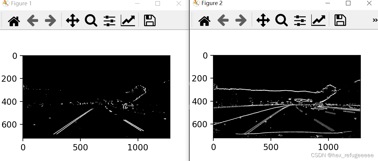

1.2 使用颜色阈值检测

使用图像中的rgb中不同数字进行检测提取。

def rgb_select(img,r_thresh,g_thresh,b_thresh):r_channel = img[:,:,0]g_channel = img[:,:,1]b_channel = img[:,:,2]r_binary = np.zeros_like(r_channel)r_binary[(r_channel > r_thresh[0]) & (r_channel <= r_thresh[1])] = 1g_binary = np.zeros_like(g_channel)g_binary[(g_channel > g_thresh[0]) & (g_channel <= g_thresh[1])] = 1b_binary = np.zeros_like(b_channel)b_binary[(b_channel > b_thresh[0]) & (b_channel <= b_thresh[1])] = 1#combined = np.zeros_like(r_channel)combined[((r_binary == 1) & (g_binary == 1) & (b_binary == 1))] = 1return combined

在函数rbg_select中分别划分不同的rgb通道的数组，然后创建不同的新的数组，并将符合阈值内的点设置为1，最后将它们合并起来输出为图像combined。

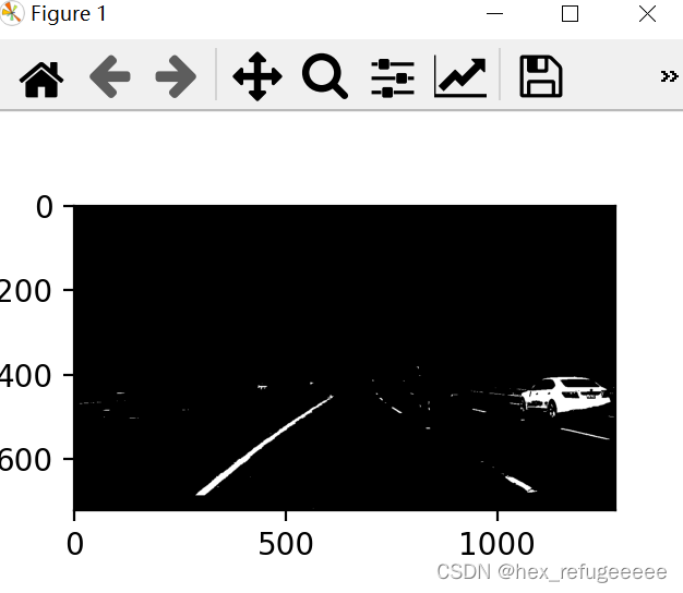
 1.3 融合sobel和rgb的边缘检测

就是将两个图像中值为1的合并起来，容易实现。

def color_gradient_threshold(image):ksize = 15gradx = abs_sobel_thresh(image,orient='x',sobel_kernel=ksize,thresh=(50,180))rgb_binary = rgb_select(image,r_thresh=(225,255),g_thresh=(180,255),b_thresh=(0,255))combined_binary = np.zeros_like(image)combined_binary[((gradx==1)|(rgb_binary==1))] = 255color_binary = combined_binaryreturn color_binary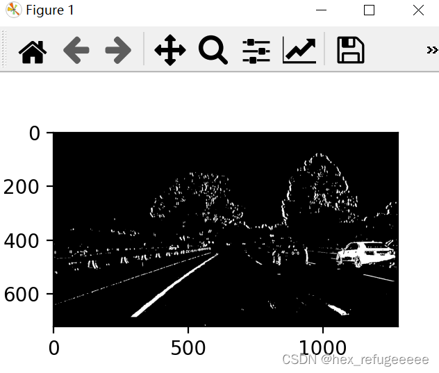

 1.4 小结

边缘检测效果完成，因为是基于Carla做的车道线边缘检测，而Carla中输出的图像输出的效果比较理想，所以直接使用sobel和rgb边缘检测融合就可以达到很好的效果所以没有做过多的研究，实际情况比较复杂可能并不适用。

二、选择车道线的区域

这里要注意用数组表示图像的时候原点一般是左上角，向右为x轴正方向，向下为y轴正方向。

所以先选择出左下角，右下角：

    ksize = 15img_color = color_gradient_threshold(image)left_bottom = [0, img_color.shape[0]]right_bottom = [img_color.shape[1],img_color.shape[0]]

选择另外一个顶点：

    apex = [ img_color.shape[1]/2, 420 ]vertices = np.array([ left_bottom, right_bottom, apex ],np.int32)

其中vertices存储的是三个点，分别是左下角、右下角和顶点。

接下来使用刚刚选择的点与边缘检测后的图像按位与得到选择车道线的区域：

def region_of_interest(img,vertices):mask = np.zeros_like(img)cv2.fillPoly(mask,[vertices],[255,255,255])masked_image = cv2.bitwise_and(img,mask)return masked_image

其中函数fillPoly函数第一个参数表示为原始图像，第二个参数为选择的点，第三个参数表示为赋值为白色。

而bitwise_and是将两个参数按位与。

最后输出按位与后的图像。

 效果还可以。

三、投影变换

将原先小的三角形区域利用投影变换成大的区域。

主要运用cv中的透视变换：

def perspective_transform(image):# give 4 points as original coordinates.top_left =[590,460]top_right = [750,460]bottom_left = [330,650]bottom_right =  [1130,650]# give 4 points to project.proj_top_left = [250,100]proj_top_right = [1150,100]proj_bottom_left  =  [330,650]proj_bottom_right =  [1130,650]# to get image size.img_size = (image.shape[1],image.shape[0])# pts1 = np.float32([top_left,top_right,bottom_left,bottom_right])pts2 = np.float32([proj_top_left,proj_top_right,proj_bottom_left,proj_bottom_right])matrix_K = cv2.getPerspectiveTransform(pts1,pts2)img_k = cv2.warpPerspective(image,matrix_K,img_size)return img_k

先划定四个点分别是左上、右上、左下和右下，为原始图像区域，

在划定投影区域。

运用函数getPerspectiveTransform它的第一个参数为平面1，第二个参数为平面2，求出平面1上的点要映射到平面2上所需要的变换的矩阵。

函数warpPerspective它的第一个参数为原始图像，第二个参数为投影变换矩阵，第三个参数为输出图像的大小，这里使用的就是原始图像的大小，需要注意一般为宽在前，长在后。

最后输出的就是变换后的图像信息。

 四、车道线提取

4.1 直方图显示

使用直方图来显示前面拉伸后的图像信息。

def histogram_img(image):histogram_binary = np.zeros((image.shape[0],image.shape[1]),dtype=np.int)histogram_binary[image[:,:,0]>0] = 1histogram = np.sum(histogram_binary[:,:],axis=0)print("histogram: ",histogram)print("histogram shape: ",histogram.shape)return histogram 

代码比较容易理解，设置一个同输入图像同尺寸的数组，将原来图像中任一rgb信息大于0的位置赋值为1，其实设置为255也可以，因为前面设置的就是255。之后就将它按列累加起来，返回这一行累加的数组（1*n）。

 4.2 车道线定位

获得的前面的直方图后，求出它的两个波峰的位置来获得车道线的大概位置。

def lane_position(histogram):histogram_size = histogram.shapemiddle_point = int(histogram_size[0]/2)print("middle_point: ",middle_point)#left_point = [0,0]for i in range(middle_point):# 寻找直方图中的波峰即顶点if histogram[i] > left_point[1]:left_point[1] = histogram[i]left_point[0] = i#right_point = [0,0]for j in range(middle_point,histogram_size[0]):if histogram[j] > right_point[1]:right_point[1] = histogram[j]right_point[0] = jresult_points = [left_point,right_point]           print("result_points: ",result_points)return result_points

输出位置：
result_points:  [[342, 566], [1014, 291]]

说明两个车道线大概在这两个点附近。

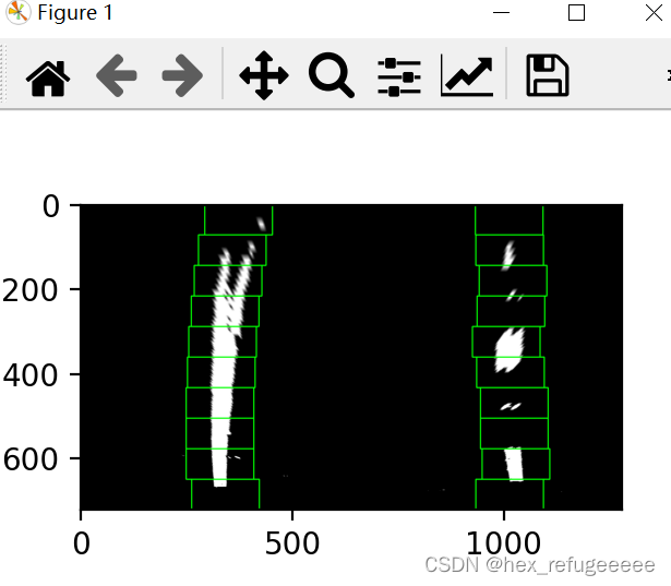
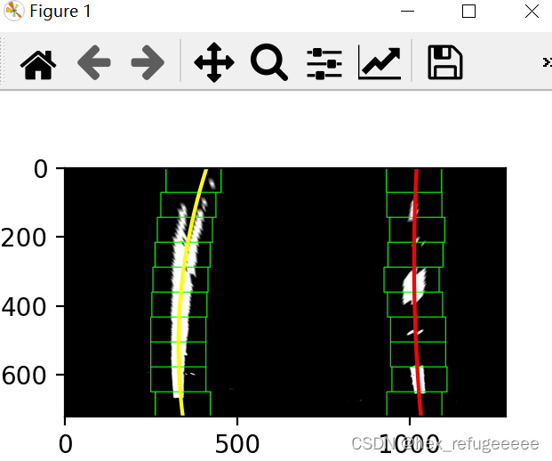
4.3 滑动窗口

将前面求得的两个坐标为起点来构建滑动窗口将车道线包裹在内。

def sliding_window(image,lanes_pos):# starting original points for windows.left_x_current = lanes_pos[0][0]right_x_current = lanes_pos[1][0]nWindows = 10window_height = np.int(image.shape[0]//nWindows)window_width = 80# to get the non-zero data in the input image.nonzero = image.nonzero() nonzero_y = nonzero[0]nonzero_x = nonzero[1]## create a empty list to receive left/right line pixel.left_lane_inds = []right_lane_inds = []# create window by windowfor window in range(nWindows):# window size.win_y_top = image.shape[0] - (window +1)*window_heightwin_y_bottom = image.shape[0] - window*window_heightwin_x_left_left = left_x_current - window_widthwin_x_left_right = left_x_current + window_width win_x_right_left = right_x_current - window_widthwin_x_right_right = right_x_current + window_width# define a rectangle for left+right lane.# and add the rectangle to the input image.cv2.rectangle(image,(win_x_left_left,win_y_top),(win_x_left_right,win_y_bottom),(0,255,0),2)cv2.rectangle(image,(win_x_right_left,win_y_top),(win_x_right_right,win_y_bottom),(0,255,0),2)good_left_inds = ((nonzero_y >= win_y_top)&(nonzero_y < win_y_bottom)&(nonzero_x >= win_x_left_left)&(nonzero_x < win_x_left_right)).nonzero()[0]good_right_inds = ((nonzero_y >= win_y_top)&(nonzero_y < win_y_bottom)&(nonzero_x >= win_x_right_left)&(nonzero_x < win_x_right_right)).nonzero()[0]#print(good_left_inds)left_lane_inds.append(good_left_inds)right_lane_inds.append(good_right_inds)##print("nonzero_x_left:",nonzero_x[good_left_inds])#print("non_zero_x_right:",nonzero_x[good_right_inds])if len(good_left_inds)>50:left_x_current = np.int(np.mean(nonzero_x[good_left_inds]))if len(good_right_inds)>50:right_x_current = np.int(np.mean(nonzero_x[good_right_inds]))# ending of lop.#print("left_lane_inds",left_lane_inds)# to transfom a list of list to a list.left_lane_inds = np.concatenate(left_lane_inds)right_lane_inds = np.concatenate(right_lane_inds)#print("left_lane_inds",left_lane_inds)left_x = nonzero_x[left_lane_inds]left_y = nonzero_y[left_lane_inds]right_x = nonzero_x[right_lane_inds]right_y = nonzero_y[right_lane_inds]#results = [image,left_x,left_y,right_x,right_y]#print("sliding windows results: ",results)return results

代码写的很明白，首先去输入的坐标为左边的车道线x坐标和右边车道线y坐标，

然后计算滑动窗口的高度和宽度，

算出图像中所有不唯1的坐标，将它们放入nonzero数组中，

分别取行数为nonzero_y和列数为nonzero_x，

之后就是在for循环不断的画出矩形，利用rectangle函数进行绘制图像。

然后计算这个窗口里面大于1的数的位置平均值为下一个窗口的中间值，

最后保存所有的大于1的坐标，并于图像一并返回。

 4.4 曲线拟合

构建出一条曲线来表示车道线，方便之后利用曲线的曲率来控制车辆的转向信息。

具体实现为将之前获得的图像中所有的白色点的坐标，将它们进行拟合成曲线。

def fit_polynominal(img_sliding_window):image = img_sliding_window[0]left_x = img_sliding_window[1]left_y = img_sliding_window[2]right_x = img_sliding_window[3]right_y = img_sliding_window[4]left_fit = np.polyfit(left_y,left_x,2)right_fit = np.polyfit(right_y,right_x,2)# to generate x and y values for plotting.ploty = np.linspace(0,image.shape[0]-1,image.shape[0])left_fitx = left_fit[0]*ploty**2 + left_fit[1]*ploty + left_fit[2]right_fitx = right_fit[0]*ploty**2 + right_fit[1]*ploty + right_fit[2]plt.plot(left_fitx,ploty,color='yellow')plt.plot(right_fitx,ploty,color='red')return 0

其中主要函数为polyfit函数它将参数一和参数二进行二次曲线拟合，拟合后得到三个参数存在返回值里面。

之后依据高度进行划分点，然后更具拟合后的参数构造曲线方程，最后输出到图像上。

 4.5 添加蒙版

通过前面获得的两条曲线的坐标点，在两条曲线之间添加一层蒙版，表示车道位置。

def drawing_poly(img_ori, img_fit):# create an image to draw the lines on.#left_fitx = img_fit[0]right_fitx = img_fit[1]ploty = img_fit[2]#img_zero = np.zeros_like(img_ori)##print("left_fitx:",left_fitx)#print("ploty:",ploty)pts_left = np.transpose(np.vstack([left_fitx,ploty]))#print("pts_left:",pts_left)# print("pts_left shape:",pts_left.shape)pts_right = np.transpose(np.vstack([right_fitx,ploty]))pts_right = np.flipud(pts_right)#print("pts_right:",pts_right)#print("pts_right shape:",pts_right.shape)pts = np.vstack((pts_left,pts_right))#print("pts_left+right:",pts)#print("pts_left+right shape:",pts.shape)img_mask = cv2.fillPoly(img_zero,np.int_([pts]),(0,255,0))#print("img_mask:",img_mask)#print("img_mask shape:",img_mask.shape)return img_mask

主要是对于右侧坐标的反转，

pts_right = np.flipud(pts_right)是为了后面绘制多边形的时候连线准确，

pts = np.vstack((pts_left,pts_right))

img_mask = cv2.fillPoly(img_zero,np.int_([pts]),(0,255,0))

 4.6 反向映射

将之前的处理后的图像反向映射回原始图像。

将之前的代码中的参数变换位置就可以获得反过来的变换矩阵。

getPerspectiveTransform

def drawing_poly_perspective_back(img_ori, img_fit,matrix_K_back):# create an image to draw the lines on.#left_fitx = img_fit[0]right_fitx = img_fit[1]ploty = img_fit[2]#img_zero = np.zeros_like(img_ori)##print("left_fitx:",left_fitx)#print("ploty:",ploty)pts_left = np.transpose(np.vstack([left_fitx,ploty]))#print("pts_left:",pts_left)#print("pts_left shape:",pts_left.shape)pts_right = np.transpose(np.vstack([right_fitx,ploty]))pts_right = np.flipud(pts_right)#print("pts_right:",pts_right)#print("pts_right shape:",pts_right.shape)pts = np.vstack((pts_left,pts_right))#print("pts_left+right:",pts)#print("pts_left+right shape:",pts.shape)img_mask = cv2.fillPoly(img_zero,np.int_([pts]),(0,255,0))#print("img_mask:",img_mask)#print("img_mask shape:",img_mask.shape)# to get image size.img_size = (img_ori.shape[1],img_ori.shape[0])img_mask_back = cv2.warpPerspective(img_mask,matrix_K_back,img_size)return img_mask_back

五、视频输入

 车道线检测变换基本完成，在将单帧图像修改为视频进行计算。

    # video input.video_input = "./test_video/project_video.mp4"cap = cv2.VideoCapture(video_input)# output setting.video_output = "./test_video/project_video_output_v2.mp4"fourcc = cv2.VideoWriter_fourcc(*'mp4v')width = 1280height = 720fps = 20video_out = cv2.VideoWriter(video_output,fourcc,fps,(width,height))# add some text to the output video.content = "this is frame: "pos = (64,90)color = (0,255,0)font = cv2.FONT_HERSHEY_SIMPLEXweight = 2size = 1count = 0## prcessing frame by frame. while True:ret,frame = cap.read()if not ret:print("video read error, exited...")breakif cv2.waitKey(25) & 0xFF == ord('q'):print(" you quit the program by clicking 'q'...")breakimage = frameksize = 15img_color = color_gradient_threshold(image)#left_bottom = [0, img_color.shape[0]]right_bottom = [img_color.shape[1],img_color.shape[0]]apex = [ img_color.shape[1]/2, 420 ]vertices = np.array([ left_bottom, right_bottom, apex ],np.int32)img_interest = region_of_interest(img_color,vertices)img_perspective,matrix_K_back = perspective_transform(img_interest)img_histogram = histogram_img(img_perspective)lanes_pos = lane_position(img_histogram)img_sliding_window = sliding_window(img_perspective,lanes_pos) img_fit_list = fit_polynominal(img_sliding_window)## to set the transparency of img.img_mask_back = drawing_poly_perspective_back(image,img_fit_list,matrix_K_back)#img_mask_back_result = img_mask_back*0.5 + image*0.5img_mask_back_result = cv2.addWeighted(image,1,img_mask_back,0.3,0)results = img_mask_back_resultcontents = content + str(count)cv2.putText(results,contents,pos,font,size,color,weight,cv2.LINE_AA)cv2.imshow("frame",results)video_out.write(results)#count += 1cap.release()cv2.destroyAllWindows()

容易理解，不做解读，

但只能达到一个简单的车道线识别效果，而且处理速度很慢，遇到颜色变化不明显的会直接error，在具体的项目应用中需要改进，改进在后面的文章中体现。

参考文章：

（六）高级车道线识别 - 知乎在之前的文章中，我们介绍了利用opencv进行简单的车道线识别项目，本文将更进一步，对相对复杂场景下的车道线进行识别。具体来讲，本文在简单车道线项目的基础上增加了如下知识点：颜色空间，透视变换，滑移窗，弯…https://zhuanlan.zhihu.com/p/56712138实操：自动驾驶的车道识别原理及演练（附代码下载）大家五一快乐呀，我是李慢慢。前情提要距离上一次正儿八经发文，貌似已经过去两个月了，因为疫情原因我一直都是居家https://mp.weixin.qq.com/s/9ykWyXsCnTVqyojRlb7H9A