人工神经网络

感知机

1．感知机是根据输入实例的特征向量$x$对其进行二类分类的线性分类模型：

$$f(x)=\mathrm{sign}(w\cdot x+b)$$

感知机模型对应于输入空间（特征空间）中的分离超平面$w\cdot x+b=0$。

2．感知机学习的策略是极小化损失函数：

$$\underset{w,b}{\min }L(w,b)=-\sum _{x_i\in M}{y}_i\left(w\cdot x_i+b\right)$$

损失函数对应于误分类点到分离超平面的总距离。

3．感知机学习算法是基于随机梯度下降法的对损失函数的最优化算法，有原始形式和对偶形式。算法简单且易于实现。原始形式中，首先任意选取一个超平面，然后用梯度下降法不断极小化目标函数。在这个过程中一次随机选取一个误分类点使其梯度下降。

4．当训练数据集线性可分时，感知机学习算法是收敛的。感知机算法在训练数据集上的误分类次数$k$满足不等式：

$$k⩽{\left(\frac{R}{\gamma }\right)}^2$$

当训练数据集线性可分时，感知机学习算法存在无穷多个解，其解由于不同的初值或不同的迭代顺序而可能有所不同。

二分类模型

$f(x)=sign(w\cdot x+b)$

$\mathrm{sign}(x)=\{\begin{array}{ll}+1,& x⩾0\\ -1,& x<0\end{array}$

给定训练集：

T = { ( x 1 , y 1 ) , ( x 2 , y 2 ) , ⋯ , ( x N , y N ) } T=\left\{\left(x_{1}, y_{1}\right),\left(x_{2}, y_{2}\right), \cdots,\left(x_{N}, y_{N}\right)\right\} T={(x1​,y1​),(x2​,y2​),⋯,(xN​,yN​)}

定义感知机的损失函数

$L(w,b)=-{\sum }_{x_i\in M}{y}_i\left(w\cdot x_i+b\right)$

---

算法

随即梯度下降法 Stochastic Gradient Descent

随机抽取一个误分类点使其梯度下降。

$w=w+\eta y_i{x}_i$

$b=b+\eta y_i$

当实例点被误分类，即位于分离超平面的错误侧，则调整$w$, $b$的值，使分离超平面向该无分类点的一侧移动，直至误分类点被正确分类

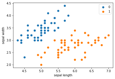
拿出iris数据集中两个分类的数据和[sepal length，sepal width]作为特征

1. 基于手写代码的感知器模型

1.1 数据读取

import pandas as pd
import numpy as np
from sklearn.datasets import load_iris
import matplotlib.pyplot as plt
%matplotlib inline

# load data
iris = load_iris()
iris

{'data': array([[5.1, 3.5, 1.4, 0.2],[4.9, 3. , 1.4, 0.2],[4.7, 3.2, 1.3, 0.2],[4.6, 3.1, 1.5, 0.2],[5. , 3.6, 1.4, 0.2],[5.4, 3.9, 1.7, 0.4],[4.6, 3.4, 1.4, 0.3],[5. , 3.4, 1.5, 0.2],[4.4, 2.9, 1.4, 0.2],[4.9, 3.1, 1.5, 0.1],[5.4, 3.7, 1.5, 0.2],[4.8, 3.4, 1.6, 0.2],[4.8, 3. , 1.4, 0.1],[4.3, 3. , 1.1, 0.1],[5.8, 4. , 1.2, 0.2],[5.7, 4.4, 1.5, 0.4],[5.4, 3.9, 1.3, 0.4],[5.1, 3.5, 1.4, 0.3],[5.7, 3.8, 1.7, 0.3],[5.1, 3.8, 1.5, 0.3],[5.4, 3.4, 1.7, 0.2],[5.1, 3.7, 1.5, 0.4],[4.6, 3.6, 1. , 0.2],[5.1, 3.3, 1.7, 0.5],[4.8, 3.4, 1.9, 0.2],[5. , 3. , 1.6, 0.2],[5. , 3.4, 1.6, 0.4],[5.2, 3.5, 1.5, 0.2],[5.2, 3.4, 1.4, 0.2],[4.7, 3.2, 1.6, 0.2],[4.8, 3.1, 1.6, 0.2],[5.4, 3.4, 1.5, 0.4],[5.2, 4.1, 1.5, 0.1],[5.5, 4.2, 1.4, 0.2],[4.9, 3.1, 1.5, 0.2],[5. , 3.2, 1.2, 0.2],[5.5, 3.5, 1.3, 0.2],[4.9, 3.6, 1.4, 0.1],[4.4, 3. , 1.3, 0.2],[5.1, 3.4, 1.5, 0.2],[5. , 3.5, 1.3, 0.3],[4.5, 2.3, 1.3, 0.3],[4.4, 3.2, 1.3, 0.2],[5. , 3.5, 1.6, 0.6],[5.1, 3.8, 1.9, 0.4],[4.8, 3. , 1.4, 0.3],[5.1, 3.8, 1.6, 0.2],[4.6, 3.2, 1.4, 0.2],[5.3, 3.7, 1.5, 0.2],[5. , 3.3, 1.4, 0.2],[7. , 3.2, 4.7, 1.4],[6.4, 3.2, 4.5, 1.5],[6.9, 3.1, 4.9, 1.5],[5.5, 2.3, 4. , 1.3],[6.5, 2.8, 4.6, 1.5],[5.7, 2.8, 4.5, 1.3],[6.3, 3.3, 4.7, 1.6],[4.9, 2.4, 3.3, 1. ],[6.6, 2.9, 4.6, 1.3],[5.2, 2.7, 3.9, 1.4],[5. , 2. , 3.5, 1. ],[5.9, 3. , 4.2, 1.5],[6. , 2.2, 4. , 1. ],[6.1, 2.9, 4.7, 1.4],[5.6, 2.9, 3.6, 1.3],[6.7, 3.1, 4.4, 1.4],[5.6, 3. , 4.5, 1.5],[5.8, 2.7, 4.1, 1. ],[6.2, 2.2, 4.5, 1.5],[5.6, 2.5, 3.9, 1.1],[5.9, 3.2, 4.8, 1.8],[6.1, 2.8, 4. , 1.3],[6.3, 2.5, 4.9, 1.5],[6.1, 2.8, 4.7, 1.2],[6.4, 2.9, 4.3, 1.3],[6.6, 3. , 4.4, 1.4],[6.8, 2.8, 4.8, 1.4],[6.7, 3. , 5. , 1.7],[6. , 2.9, 4.5, 1.5],[5.7, 2.6, 3.5, 1. ],[5.5, 2.4, 3.8, 1.1],[5.5, 2.4, 3.7, 1. ],[5.8, 2.7, 3.9, 1.2],[6. , 2.7, 5.1, 1.6],[5.4, 3. , 4.5, 1.5],[6. , 3.4, 4.5, 1.6],[6.7, 3.1, 4.7, 1.5],[6.3, 2.3, 4.4, 1.3],[5.6, 3. , 4.1, 1.3],[5.5, 2.5, 4. , 1.3],[5.5, 2.6, 4.4, 1.2],[6.1, 3. , 4.6, 1.4],[5.8, 2.6, 4. , 1.2],[5. , 2.3, 3.3, 1. ],[5.6, 2.7, 4.2, 1.3],[5.7, 3. , 4.2, 1.2],[5.7, 2.9, 4.2, 1.3],[6.2, 2.9, 4.3, 1.3],[5.1, 2.5, 3. , 1.1],[5.7, 2.8, 4.1, 1.3],[6.3, 3.3, 6. , 2.5],[5.8, 2.7, 5.1, 1.9],[7.1, 3. , 5.9, 2.1],[6.3, 2.9, 5.6, 1.8],[6.5, 3. , 5.8, 2.2],[7.6, 3. , 6.6, 2.1],[4.9, 2.5, 4.5, 1.7],[7.3, 2.9, 6.3, 1.8],[6.7, 2.5, 5.8, 1.8],[7.2, 3.6, 6.1, 2.5],[6.5, 3.2, 5.1, 2. ],[6.4, 2.7, 5.3, 1.9],[6.8, 3. , 5.5, 2.1],[5.7, 2.5, 5. , 2. ],[5.8, 2.8, 5.1, 2.4],[6.4, 3.2, 5.3, 2.3],[6.5, 3. , 5.5, 1.8],[7.7, 3.8, 6.7, 2.2],[7.7, 2.6, 6.9, 2.3],[6. , 2.2, 5. , 1.5],[6.9, 3.2, 5.7, 2.3],[5.6, 2.8, 4.9, 2. ],[7.7, 2.8, 6.7, 2. ],[6.3, 2.7, 4.9, 1.8],[6.7, 3.3, 5.7, 2.1],[7.2, 3.2, 6. , 1.8],[6.2, 2.8, 4.8, 1.8],[6.1, 3. , 4.9, 1.8],[6.4, 2.8, 5.6, 2.1],[7.2, 3. , 5.8, 1.6],[7.4, 2.8, 6.1, 1.9],[7.9, 3.8, 6.4, 2. ],[6.4, 2.8, 5.6, 2.2],[6.3, 2.8, 5.1, 1.5],[6.1, 2.6, 5.6, 1.4],[7.7, 3. , 6.1, 2.3],[6.3, 3.4, 5.6, 2.4],[6.4, 3.1, 5.5, 1.8],[6. , 3. , 4.8, 1.8],[6.9, 3.1, 5.4, 2.1],[6.7, 3.1, 5.6, 2.4],[6.9, 3.1, 5.1, 2.3],[5.8, 2.7, 5.1, 1.9],[6.8, 3.2, 5.9, 2.3],[6.7, 3.3, 5.7, 2.5],[6.7, 3. , 5.2, 2.3],[6.3, 2.5, 5. , 1.9],[6.5, 3. , 5.2, 2. ],[6.2, 3.4, 5.4, 2.3],[5.9, 3. , 5.1, 1.8]]),'target': array([0, 0, 0, 0, 0, 0, 0, 0, 0, 0, 0, 0, 0, 0, 0, 0, 0, 0, 0, 0, 0, 0,0, 0, 0, 0, 0, 0, 0, 0, 0, 0, 0, 0, 0, 0, 0, 0, 0, 0, 0, 0, 0, 0,0, 0, 0, 0, 0, 0, 1, 1, 1, 1, 1, 1, 1, 1, 1, 1, 1, 1, 1, 1, 1, 1,1, 1, 1, 1, 1, 1, 1, 1, 1, 1, 1, 1, 1, 1, 1, 1, 1, 1, 1, 1, 1, 1,1, 1, 1, 1, 1, 1, 1, 1, 1, 1, 1, 1, 2, 2, 2, 2, 2, 2, 2, 2, 2, 2,2, 2, 2, 2, 2, 2, 2, 2, 2, 2, 2, 2, 2, 2, 2, 2, 2, 2, 2, 2, 2, 2,2, 2, 2, 2, 2, 2, 2, 2, 2, 2, 2, 2, 2, 2, 2, 2, 2, 2]),'frame': None,'target_names': array(['setosa', 'versicolor', 'virginica'], dtype='<U10'),'DESCR': '.. _iris_dataset:\n\nIris plants dataset\n--------------------\n\n**Data Set Characteristics:**\n\n    :Number of Instances: 150 (50 in each of three classes)\n    :Number of Attributes: 4 numeric, predictive attributes and the class\n    :Attribute Information:\n        - sepal length in cm\n        - sepal width in cm\n        - petal length in cm\n        - petal width in cm\n        - class:\n                - Iris-Setosa\n                - Iris-Versicolour\n                - Iris-Virginica\n                \n    :Summary Statistics:\n\n    ============== ==== ==== ======= ===== ====================\n                    Min  Max   Mean    SD   Class Correlation\n    ============== ==== ==== ======= ===== ====================\n    sepal length:   4.3  7.9   5.84   0.83    0.7826\n    sepal width:    2.0  4.4   3.05   0.43   -0.4194\n    petal length:   1.0  6.9   3.76   1.76    0.9490  (high!)\n    petal width:    0.1  2.5   1.20   0.76    0.9565  (high!)\n    ============== ==== ==== ======= ===== ====================\n\n    :Missing Attribute Values: None\n    :Class Distribution: 33.3% for each of 3 classes.\n    :Creator: R.A. Fisher\n    :Donor: Michael Marshall (MARSHALL%PLU@io.arc.nasa.gov)\n    :Date: July, 1988\n\nThe famous Iris database, first used by Sir R.A. Fisher. The dataset is taken\nfrom Fisher\'s paper. Note that it\'s the same as in R, but not as in the UCI\nMachine Learning Repository, which has two wrong data points.\n\nThis is perhaps the best known database to be found in the\npattern recognition literature.  Fisher\'s paper is a classic in the field and\nis referenced frequently to this day.  (See Duda & Hart, for example.)  The\ndata set contains 3 classes of 50 instances each, where each class refers to a\ntype of iris plant.  One class is linearly separable from the other 2; the\nlatter are NOT linearly separable from each other.\n\n.. topic:: References\n\n   - Fisher, R.A. "The use of multiple measurements in taxonomic problems"\n     Annual Eugenics, 7, Part II, 179-188 (1936); also in "Contributions to\n     Mathematical Statistics" (John Wiley, NY, 1950).\n   - Duda, R.O., & Hart, P.E. (1973) Pattern Classification and Scene Analysis.\n     (Q327.D83) John Wiley & Sons.  ISBN 0-471-22361-1.  See page 218.\n   - Dasarathy, B.V. (1980) "Nosing Around the Neighborhood: A New System\n     Structure and Classification Rule for Recognition in Partially Exposed\n     Environments".  IEEE Transactions on Pattern Analysis and Machine\n     Intelligence, Vol. PAMI-2, No. 1, 67-71.\n   - Gates, G.W. (1972) "The Reduced Nearest Neighbor Rule".  IEEE Transactions\n     on Information Theory, May 1972, 431-433.\n   - See also: 1988 MLC Proceedings, 54-64.  Cheeseman et al"s AUTOCLASS II\n     conceptual clustering system finds 3 classes in the data.\n   - Many, many more ...','feature_names': ['sepal length (cm)','sepal width (cm)','petal length (cm)','petal width (cm)'],'filename': 'iris.csv','data_module': 'sklearn.datasets.data'}

# load data
iris = load_iris()
df = pd.DataFrame(iris.data, columns=iris.feature_names)
df['label'] = iris.target

df.head()

	sepal length (cm)	sepal width (cm)	petal length (cm)	petal width (cm)	label
0	5.1	3.5	1.4	0.2	0
1	4.9	3.0	1.4	0.2	0
2	4.7	3.2	1.3	0.2	0
3	4.6	3.1	1.5	0.2	0
4	5.0	3.6	1.4	0.2	0

df.columns=["sepal length","sepal width","petal length","petal width","label"]

#查看标签元素列的元素种类和个数
df["label"].value_counts()

0    50
1    50
2    50
Name: label, dtype: int64

plt.scatter(df[:50]['sepal length'], df[:50]['sepal width'], label='0')
plt.scatter(df[50:100]['sepal length'], df[50:100]['sepal width'], label='1')
plt.xlabel('sepal length')
plt.ylabel('sepal width')
plt.legend()

<matplotlib.legend.Legend at 0x215d7f87f40>

data = np.array(df.iloc[:100, [0, 1, -1]])

X, y = data[:,:-1], data[:,-1]

data[:,-1]

array([0., 0., 0., 0., 0., 0., 0., 0., 0., 0., 0., 0., 0., 0., 0., 0., 0.,0., 0., 0., 0., 0., 0., 0., 0., 0., 0., 0., 0., 0., 0., 0., 0., 0.,0., 0., 0., 0., 0., 0., 0., 0., 0., 0., 0., 0., 0., 0., 0., 0., 1.,1., 1., 1., 1., 1., 1., 1., 1., 1., 1., 1., 1., 1., 1., 1., 1., 1.,1., 1., 1., 1., 1., 1., 1., 1., 1., 1., 1., 1., 1., 1., 1., 1., 1.,1., 1., 1., 1., 1., 1., 1., 1., 1., 1., 1., 1., 1., 1., 1.])

y = np.array([1 if i == 1 else -1 for i in y])

y

array([-1, -1, -1, -1, -1, -1, -1, -1, -1, -1, -1, -1, -1, -1, -1, -1, -1,-1, -1, -1, -1, -1, -1, -1, -1, -1, -1, -1, -1, -1, -1, -1, -1, -1,-1, -1, -1, -1, -1, -1, -1, -1, -1, -1, -1, -1, -1, -1, -1, -1,  1,1,  1,  1,  1,  1,  1,  1,  1,  1,  1,  1,  1,  1,  1,  1,  1,  1,1,  1,  1,  1,  1,  1,  1,  1,  1,  1,  1,  1,  1,  1,  1,  1,  1,1,  1,  1,  1,  1,  1,  1,  1,  1,  1,  1,  1,  1,  1,  1])

X[:5],y[:5]

(array([[5.1, 3.5],[4.9, 3. ],[4.7, 3.2],[4.6, 3.1],[5. , 3.6]]),array([-1, -1, -1, -1, -1]))

$w=w+\eta y_i{x}_i$

$b=b+\eta y_i$

1.2 构建感知器模型

y.shape

(100,)

class Perception_model:def __init__(self,n):self.w=np.zeros(n,dtype=np.float32)self.b=0self.l_rate=0.1def sign(self,x):y=np.dot(x,self.w)+self.breturn ydef fit(self,X_train,y_train):is_wrong=Truewhile is_wrong:is_wrong=Falsefor i in range(len(X_train)):if y_train[i]*self.sign(X_train[i])<=0:self.w=self.w+self.l_rate*np.dot(y_train[i],X_train[i])self.b=self.b+self.l_rate*y_train[i]is_wrong=True

1.3 实例化模型并训练模型

model=Perception_model(X.shape[1])
model.fit(X,y)

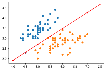
1.4 可视化

np.max(X[:,0]),np.min(X[:,0])

(7.0, 4.3)

X_fig=np.arange(int(np.min(X[:,0])),int(np.max(X[:,0])+1),0.5)
X_fig
#w[0]*x1+w[1]*x2+b=0

array([4. , 4.5, 5. , 5.5, 6. , 6.5, 7. , 7.5])

y1=-(model.w[0]*X_fig+model.b)/model.w[1]
plt.plot(X_fig,y1,"r-+")
plt.scatter(X[:50,0],X[:50,1],label=0)
plt.scatter(X[50:100,0],X[50:100,1],label=1)
plt.show()

2. 基于sklearn的感知器实现

2.1 数据获取与前面相同

2.2 导入类库

from sklearn.linear_model import Perceptron

2.3 实例化感知器

model=Perceptron(fit_intercept=True,max_iter=1000,shuffle=True)

2.4 采用数据拟合感知器

model.fit(X,y)

Perceptron()

model.coef_

array([[ 23.2, -38.7]])

model.intercept_

array([-5.])

2.5 可视化

# 画布大小
plt.figure(figsize=(6,4))# 中文标题
plt.rcParams['font.sans-serif'] = ['SimHei']
plt.rcParams['axes.unicode_minus'] = False
plt.title('鸢尾花线性数据示例')X_fig=np.arange(int(np.min(X[:,0])),int(np.max(X[:,0])+1),0.5)
X_fig
y1=-(model.coef_[0][0]*X_fig+model.intercept_)/model.coef_[0][1]
plt.plot(X_fig,y1,"r-+")
plt.scatter(X[:50,0],X[:50,1],label=0)
plt.scatter(X[50:100,0],X[50:100,1],label=1)plt.legend()  # 显示图例
plt.grid(False)  # 不显示网格
plt.xlabel('sepal length')
plt.ylabel('sepal width')
plt.legend()
plt.show()

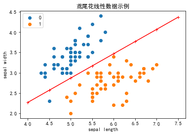
注意 !

在上图中，有一个位于左下角的蓝点没有被正确分类，这是因为 SKlearn 的 Perceptron 实例中有一个tol参数。

tol 参数规定了如果本次迭代的损失和上次迭代的损失之差小于一个特定值时，停止迭代。所以我们需要设置 tol=None 使之可以继续迭代：

model=Perceptron(fit_intercept=True,max_iter=1000,shuffle=True,tol=None)
model.fit(X,y)

Perceptron(tol=None)

# 画布大小
plt.figure(figsize=(6,4))# 中文标题
plt.rcParams['font.sans-serif'] = ['SimHei']
plt.rcParams['axes.unicode_minus'] = False
plt.title('鸢尾花线性数据示例')X_fig=np.arange(int(np.min(X[:,0])),int(np.max(X[:,0])+1),0.5)
X_fig
y1=-(model.coef_[0][0]*X_fig+model.intercept_)/model.coef_[0][1]
plt.plot(X_fig,y1,"r-+")
plt.scatter(X[:50,0],X[:50,1],label=0)
plt.scatter(X[50:100,0],X[50:100,1],label=1)plt.legend()  # 显示图例
plt.grid(False)  # 不显示网格
plt.xlabel('sepal length')
plt.ylabel('sepal width')
plt.legend()
plt.show()

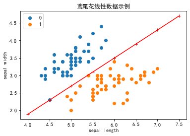
现在可以看到，所有的两种鸢尾花都被正确分类了。

实验1 将上面数据划分为训练数据和测试数据，并在Perpetron_model类中定义score函数，训练后利用score函数来输出测试分数

1. 数据读取

import pandas as pd
import numpy as np
from sklearn.datasets import load_iris
import matplotlib.pyplot as plt
%matplotlib inline

# load data
iris = load_iris()
df = pd.DataFrame(iris.data, columns=iris.feature_names)
df['label'] = iris.target

df.columns=["sepal length","sepal width","petal length","petal width","label"]
data = np.array(df.iloc[:100, [0, 1, -1]])
X, y = data[:,:-1], data[:,-1]
y = np.array([1 if i == 1 else -1 for i in y])

2. 划分训练数据和测试数据

from sklearn.model_selection import train_test_split

划分训练数据和测试数据

X_train,X_test,y_train,y_test=train_test_split(X,y,test_size=0.2)

3. 定义感知器类

定义下面的实例方法score函数

class Perception_model:def __init__(self,n):self.w=np.zeros(n,dtype=np.float32)self.b=0self.l_rate=0.1def sign(self,x):y=np.dot(x,self.w)+self.breturn ydef fit(self,X_train,y_train):is_wrong=Truewhile is_wrong:is_wrong=Falsefor i in range(len(X_train)):if y_train[i]*self.sign(X_train[i])<=0:self.w=self.w+self.l_rate*np.dot(y_train[i],X_train[i])self.b=self.b+self.l_rate*y_train[i]is_wrong=Truedef score(self,X_test,y_test):accuracy=0for i in range(len(X_test)):if self.sign(X_test[i])<=0 and y_test[i]==-1:accuracy+=1if self.sign(X_test[i])>0 and y_test[i]==1:accuracy+=1return accuracy/len(X_test)

4. 实例化模型并训练模型

model_1=Perception_model(len(X_train[0]))
model_1.fit(X_train,y_train)

5. 测试模型

调用实例方法score函数

model_1.score(X_test,y_test)

1.0