1. 归一化
# Read data from csv
pga = pd.read_csv("pga.csv")
print(type(pga))print(pga.head())

# Normalize the data 归一化值 (x - mean) / (std)
pga.distance = (pga.distance - pga.distance.mean()) / pga.distance.std()
pga.accuracy = (pga.accuracy - pga.accuracy.mean()) / pga.accuracy.std()
print(pga.head())
plt.scatter(pga.distance, pga.accuracy)
plt.xlabel('normalized distance')
plt.ylabel('normalized accuracy')
plt.show()
2. 线性回归
from sklearn.linear_model import LinearRegression
import numpy as np# We can add a dimension to an array by using np.newaxis
print("Shape of the series:", pga.distance.shape)
print("Shape with newaxis:", pga.distance[:, np.newaxis].shape)# The X variable in LinearRegression.fit() must have 2 dimensions
lm = LinearRegression()
lm.fit(pga.distance[:, np.newaxis], pga.accuracy)
theta1 = lm.coef_[0]
print (theta1)
这段代码是一个示例,展示了如何使用np.newaxis和LinearRegression来进行线性回归。
首先,通过np.newaxis将一维数组pga.distance添加一个新的维度,从而将其转换为二维数
组。通过打印数组的形状,可以看到在添加np.newaxis之前,pga.distance是一个一维数组,形状
为(n,),而添加了np.newaxis之后,形状变为(n, 1)。
然后,创建了一个LinearRegression的实例lm。使用lm.fit()方法,将转换后的特征数据
pga.distance[:, np.newaxis]和目标数据pga.accuracy作为参数,对线性回归模型进行训练拟
合。
最后,通过lm.coef_获取训练后的模型系数(权重),并将第一个特征的系数赋值给变量
theta1。pga.distance和pga.accuracy是示例数据,你需要根据实际情况替换为你自己的数据。
3. 代价函数
# The cost function of a single variable linear model# The c
# 单变量 代价函数
def cost(theta0, theta1, x, y):# Initialize costJ = 0# The number of observationsm = len(x)# Loop through each observation# 通过每次观察进行循环for i in range(m):# Compute the hypothesis # 计算假设h = theta1 * x[i] + theta0# Add to costJ += (h - y[i])**2# Average and normalize costJ /= (2*m)return J# The cost for theta0=0 and theta1=1
print(cost(0, 1, pga.distance, pga.accuracy))theta0 = 100
theta1s = np.linspace(-3,2,100)
costs = []
for theta1 in theta1s:costs.append(cost(theta0, theta1, pga.distance, pga.accuracy))plt.plot(theta1s, costs)
plt.show()
一个简单的单变量线性回归模型的代价函数实现,并且计算了在给定一组参数theta0和theta1
的情况下的代价。在这段代码中,cost()函数接受四个参数:theta0和theta1是线性模型的参数,
x是输入特征,y是目标变量。函数的目标是计算模型的代价。
首先,初始化代价J为0。然后,通过循环遍历每个观察值,计算模型的预测值h。代价J通过累
加每个观察值的误差平方来计算。最后,将代价J除以观察值的数量的两倍,以平均和归一化代
价。在这段代码的后半部分,使用一个给定的theta0值和一组theta1值,计算每个theta1对应的代
价,并将结果存储在costs列表中。然后,使用plt.plot()将theta1s和costs进行绘制,显示出代
价函数随着theta1的变化而变化的趋势。
4. 绘制三维图
import numpy as np
from mpl_toolkits.mplot3d import Axes3D# Example of a Surface Plot using Matplotlib
# Create x an y variables
x = np.linspace(-10,10,100)
y = np.linspace(-10,10,100)# We must create variables to represent each possible pair of points in x and y
# ie. (-10, 10), (-10, -9.8), ... (0, 0), ... ,(10, 9.8), (10,9.8)
# x and y need to be transformed to 100x100 matrices to represent these coordinates
# np.meshgrid will build a coordinate matrices of x and y
X, Y = np.meshgrid(x,y)
#print(X[:5,:5],"\n",Y[:5,:5])# Compute a 3D parabola
Z = X**2 + Y**2 # Open a figure to place the plot on
fig = plt.figure()
# Initialize 3D plot
ax = fig.gca(projection='3d')
# Plot the surface
ax.plot_surface(X=X,Y=Y,Z=Z)plt.show()# Use these for your excerise
theta0s = np.linspace(-2,2,100)
theta1s = np.linspace(-2,2, 100)
COST = np.empty(shape=(100,100))
# Meshgrid for paramaters
T0S, T1S = np.meshgrid(theta0s, theta1s)
# for each parameter combination compute the cost
for i in range(100):for j in range(100):COST[i,j] = cost(T0S[0,i], T1S[j,0], pga.distance, pga.accuracy)# make 3d plot
fig2 = plt.figure()
ax = fig2.gca(projection='3d')
ax.plot_surface(X=T0S,Y=T1S,Z=COST)
plt.show() 

使用Matplotlib绘制三维图形,包括一个二次曲面图和一个代价函数的图。
首先,通过使用np.linspace()函数,创建了从-10到10的等间距的100个点,分别赋值给变量
x和y。
接下来,使用np.meshgrid()函数将x和y转换为100x100的网格矩阵,分别赋值给X和Y。这
样,X和Y矩阵中的每个元素表示一个(x, y)坐标对。
然后,根据二次曲面方程Z = X**2 + Y**2计算出Z矩阵,其中Z矩阵中的每个元素表示对应坐
标点的高度。
通过plt.figure()创建一个新的图形,并通过fig.gca(projection='3d')初始化一个三维图形
的坐标系。使用ax.plot_surface()函数绘制曲面图,其中X、Y和Z分别表示X、Y和Z矩阵。
最后,使用plt.show()显示图形。
在后半部分的代码中,首先创建了两个包含100个均匀分布数值的数组theta0s和theta1s,分
别表示theta0和theta1的取值范围。
接下来,使用np.empty()创建一个空的100x100的数组COST,用于存储代价函数的计算结果。
通过使用np.meshgrid()函数,将theta0s和theta1s转换为网格矩阵T0S和T1S。
然后,通过两个嵌套的循环遍历所有可能的参数组合,并使用cost()函数计算每个参数组合对
应的代价,并将结果存储在COST数组中。
最后,使用plt.figure()创建一个新的图形,并通过fig.gca(projection='3d')初始化一个三
维图形的坐标系。使用ax.plot_surface()函数绘制代价函数的曲面图,其中X、Y和Z分别表示
T0S、T1S和COST矩阵。使用plt.show()显示图形。
5. 求导函数
线性回归模型的偏导数公式可以通过最小化代价函数推导得到。以下是推导过程:
线性回归模型假设函数为:h(x) = theta0 + theta1 * x
代价函数为均方差函数(Mean Squared Error):J(theta0, theta1) = (1/2m) * Σ(h(x) - y)^2
其中,m 是样本数量,h(x) 是模型的预测值,y 是观测值。
为了求解最优的模型参数 theta0 和 theta1,我们需要计算代价函数对这两个参数的偏导数。
首先,计算代价函数对 theta0 的偏导数:
∂J/∂theta0 = (1/m) * Σ(h(x) - y)
然后,计算代价函数对 theta1 的偏导数:
∂J/∂theta1 = (1/m) * Σ(h(x) - y) * x
# 对 theta1 进行求导# 对 thet
def partial_cost_theta1(theta0, theta1, x, y):# Hypothesish = theta0 + theta1*x# Hypothesis minus observed times xdiff = (h - y) * x# Average to compute partial derivativepartial = diff.sum() / (x.shape[0])return partialpartial1 = partial_cost_theta1(0, 5, pga.distance, pga.accuracy)
print("partial1 =", partial1)# 对theta0 进行求导
# Partial derivative of cost in terms of theta0
def partial_cost_theta0(theta0, theta1, x, y):# Hypothesish = theta0 + theta1*x# Difference between hypothesis and observationdiff = (h - y)# Compute partial derivativepartial = diff.sum() / (x.shape[0])return partialpartial0 = partial_cost_theta0(1, 1, pga.distance, pga.accuracy)
print("partial0 =", partial0)
计算代价函数对参数theta1和theta0的偏导数。
首先,定义了一个名为partial_cost_theta1()的函数,接受四个参数:theta0和theta1是线
性模型的参数,x是输入特征,y是目标变量。这个函数用于计算代价函数对theta1的偏导数。在函
数内部,首先计算假设值h,然后计算(h-y)*x,得到假设值与观察值之间的差异乘以输入特征x。
最后,将这些差异的和除以输入特征的数量,得到对theta1的偏导数。然后,通过调用
partial_cost_theta1()函数并传入参数0和5,计算出对应的偏导数partial1。
接下来,定义了一个名为partial_cost_theta0()的函数,接受四个参数:theta0和
theta1是线性模型的参数,x是输入特征,y是目标变量。这个函数用于计算代价函数对theta0的偏
导数。在函数内部,首先计算假设值h,然后计算假设值与观察值之间的差异。最后,将这些差异
的和除以输入特征的数量,得到对theta0的偏导数。然后,通过调用partial_cost_theta0()函数
并传入参数1和1,计算出对应的偏导数partial0。
6. 梯度下降
# x is our feature vector -- distance
# y is our target variable -- accuracy
# alpha is the learning rate
# theta0 is the intial theta0
# theta1 is the intial theta1
def gradient_descent(x, y, alpha=0.1, theta0=0, theta1=0):max_epochs = 1000 # Maximum number of iterations 最大迭代次数counter = 0       # Intialize a counter 当前第几次c = cost(theta1, theta0, pga.distance, pga.accuracy)  ## Initial cost 当前代价函数costs = [c]     # Lets store each update 每次损失值都记录下来# Set a convergence threshold to find where the cost function in minimized# When the difference between the previous cost and current cost #        is less than this value we will say the parameters converged# 设置一个收敛的阈值 (两次迭代目标函数值相差没有相差多少,就可以停止了)convergence_thres = 0.000001  cprev = c + 10   theta0s = [theta0]theta1s = [theta1]# When the costs converge or we hit a large number of iterations will we stop updating# 两次间隔迭代目标函数值相差没有相差多少(说明可以停止了)while (np.abs(cprev - c) > convergence_thres) and (counter < max_epochs):cprev = c# Alpha times the partial deriviative is our updated# 先求导, 导数相当于步长update0 = alpha * partial_cost_theta0(theta0, theta1, x, y)update1 = alpha * partial_cost_theta1(theta0, theta1, x, y)# Update theta0 and theta1 at the same time# We want to compute the slopes at the same set of hypothesised parameters#             so we update after finding the partial derivatives# -= 梯度下降,+=梯度上升theta0 -= update0theta1 -= update1# Store thetastheta0s.append(theta0)theta1s.append(theta1)# Compute the new cost# 当前迭代之后,参数发生更新  c = cost(theta0, theta1, pga.distance, pga.accuracy)# Store updates,可以进行保存当前代价值costs.append(c)counter += 1   # Count# 将当前的theta0, theta1, costs值都返回去return {'theta0': theta0, 'theta1': theta1, "costs": costs}print("Theta0 =", gradient_descent(pga.distance, pga.accuracy)['theta0'])
print("Theta1 =", gradient_descent(pga.distance, pga.accuracy)['theta1'])
print("costs =", gradient_descent(pga.distance, pga.accuracy)['costs'])descend = gradient_descent(pga.distance, pga.accuracy, alpha=.01)
plt.scatter(range(len(descend["costs"])), descend["costs"])
plt.show()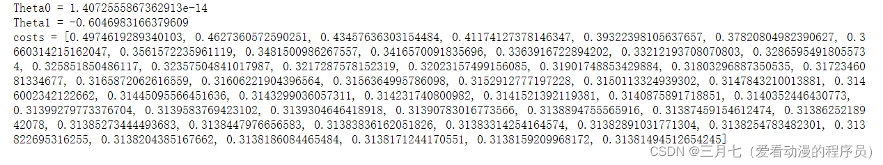

使用梯度下降法求解线性回归模型中的偏导数以及更新参数的过程。其中,gradient_descent
函数接受输入特征 x 和观测值 y,以及学习率 alpha、初始参数 theta0 和 theta1。在函数中,设
置了最大迭代次数 max_epochs 和收敛阈值 convergence_thres,用于控制算法的停止条件。初始
时,计算了初始的代价函数值 c,并将其存储在 costs 列表中。
在迭代过程中,使用偏导数的公式进行参数更新,即 theta0 -= update0 和 theta1 -=
update1。同时,计算新的代价函数值 c,并将其存储在 costs 列表中。最后,返回更新后的参数
值 theta0 和 theta1,以及代价函数值的变化过程 costs。
最后,调用了 gradient_descent 函数,并打印了最终的参数值和代价函数值。然后,绘制了
代价函数值的变化过程图。