文章目录
- 鸢尾花数据集分析
- 决策树
- K-means
鸢尾花数据集分析
决策树
# 导入机器学习相关库
from sklearn import datasets
from sklearn import treeimport matplotlib.pyplot as plt
import numpy as np# Iris数据集是常用的分类实验数据集,
# 由Fisher, 1936收集整理。Iris也称鸢尾花卉数据集,
# 是一类多重变量分析的数据集。数据集包含150个数据集,
# 分为3类,每类50个数据,每个数据包含4个属性。
# 可通过花萼长度,花萼宽度,花瓣长度,花瓣宽度4个属性预测鸢尾花卉属于(Setosa,Versicolour,Virginica)三个种类中的哪一类。
#载入数据集
iris = datasets.load_iris()
iris
{‘data’: array([[5.1, 3.5, 1.4, 0.2],
[4.9, 3. , 1.4, 0.2],
[4.7, 3.2, 1.3, 0.2],
[4.6, 3.1, 1.5, 0.2],
[5. , 3.6, 1.4, 0.2],
[5.4, 3.9, 1.7, 0.4],
[4.6, 3.4, 1.4, 0.3],
[5. , 3.4, 1.5, 0.2],
[4.4, 2.9, 1.4, 0.2],
[4.9, 3.1, 1.5, 0.1],
[5.4, 3.7, 1.5, 0.2],
[4.8, 3.4, 1.6, 0.2],
[4.8, 3. , 1.4, 0.1],
[4.3, 3. , 1.1, 0.1],
[5.8, 4. , 1.2, 0.2],
[5.7, 4.4, 1.5, 0.4],
[5.4, 3.9, 1.3, 0.4],
[5.1, 3.5, 1.4, 0.3],
[5.7, 3.8, 1.7, 0.3],
[5.1, 3.8, 1.5, 0.3],
[5.4, 3.4, 1.7, 0.2],
[5.1, 3.7, 1.5, 0.4],
[4.6, 3.6, 1. , 0.2],
[5.1, 3.3, 1.7, 0.5],
[4.8, 3.4, 1.9, 0.2],
[5. , 3. , 1.6, 0.2],
[5. , 3.4, 1.6, 0.4],
[5.2, 3.5, 1.5, 0.2],
[5.2, 3.4, 1.4, 0.2],
[4.7, 3.2, 1.6, 0.2],
[4.8, 3.1, 1.6, 0.2],
[5.4, 3.4, 1.5, 0.4],
[5.2, 4.1, 1.5, 0.1],
[5.5, 4.2, 1.4, 0.2],
[4.9, 3.1, 1.5, 0.1],
[5. , 3.2, 1.2, 0.2],
[5.5, 3.5, 1.3, 0.2],
[4.9, 3.1, 1.5, 0.1],
[4.4, 3. , 1.3, 0.2],
[5.1, 3.4, 1.5, 0.2],
[5. , 3.5, 1.3, 0.3],
[4.5, 2.3, 1.3, 0.3],
[4.4, 3.2, 1.3, 0.2],
[5. , 3.5, 1.6, 0.6],
[5.1, 3.8, 1.9, 0.4],
[4.8, 3. , 1.4, 0.3],
[5.1, 3.8, 1.6, 0.2],
[4.6, 3.2, 1.4, 0.2],
[5.3, 3.7, 1.5, 0.2],
[5. , 3.3, 1.4, 0.2],
[7. , 3.2, 4.7, 1.4],
[6.4, 3.2, 4.5, 1.5],
[6.9, 3.1, 4.9, 1.5],
[5.5, 2.3, 4. , 1.3],
[6.5, 2.8, 4.6, 1.5],
[5.7, 2.8, 4.5, 1.3],
[6.3, 3.3, 4.7, 1.6],
[4.9, 2.4, 3.3, 1. ],
[6.6, 2.9, 4.6, 1.3],
[5.2, 2.7, 3.9, 1.4],
[5. , 2. , 3.5, 1. ],
[5.9, 3. , 4.2, 1.5],
[6. , 2.2, 4. , 1. ],
[6.1, 2.9, 4.7, 1.4],
[5.6, 2.9, 3.6, 1.3],
[6.7, 3.1, 4.4, 1.4],
[5.6, 3. , 4.5, 1.5],
[5.8, 2.7, 4.1, 1. ],
[6.2, 2.2, 4.5, 1.5],
[5.6, 2.5, 3.9, 1.1],
[5.9, 3.2, 4.8, 1.8],
[6.1, 2.8, 4. , 1.3],
[6.3, 2.5, 4.9, 1.5],
[6.1, 2.8, 4.7, 1.2],
[6.4, 2.9, 4.3, 1.3],
[6.6, 3. , 4.4, 1.4],
[6.8, 2.8, 4.8, 1.4],
[6.7, 3. , 5. , 1.7],
[6. , 2.9, 4.5, 1.5],
[5.7, 2.6, 3.5, 1. ],
[5.5, 2.4, 3.8, 1.1],
[5.5, 2.4, 3.7, 1. ],
[5.8, 2.7, 3.9, 1.2],
[6. , 2.7, 5.1, 1.6],
[5.4, 3. , 4.5, 1.5],
[6. , 3.4, 4.5, 1.6],
[6.7, 3.1, 4.7, 1.5],
[6.3, 2.3, 4.4, 1.3],
[5.6, 3. , 4.1, 1.3],
[5.5, 2.5, 4. , 1.3],
[5.5, 2.6, 4.4, 1.2],
[6.1, 3. , 4.6, 1.4],
[5.8, 2.6, 4. , 1.2],
[5. , 2.3, 3.3, 1. ],
[5.6, 2.7, 4.2, 1.3],
[5.7, 3. , 4.2, 1.2],
[5.7, 2.9, 4.2, 1.3],
[6.2, 2.9, 4.3, 1.3],
[5.1, 2.5, 3. , 1.1],
[5.7, 2.8, 4.1, 1.3],
[6.3, 3.3, 6. , 2.5],
[5.8, 2.7, 5.1, 1.9],
[7.1, 3. , 5.9, 2.1],
[6.3, 2.9, 5.6, 1.8],
[6.5, 3. , 5.8, 2.2],
[7.6, 3. , 6.6, 2.1],
[4.9, 2.5, 4.5, 1.7],
[7.3, 2.9, 6.3, 1.8],
[6.7, 2.5, 5.8, 1.8],
[7.2, 3.6, 6.1, 2.5],
[6.5, 3.2, 5.1, 2. ],
[6.4, 2.7, 5.3, 1.9],
[6.8, 3. , 5.5, 2.1],
[5.7, 2.5, 5. , 2. ],
[5.8, 2.8, 5.1, 2.4],
[6.4, 3.2, 5.3, 2.3],
[6.5, 3. , 5.5, 1.8],
[7.7, 3.8, 6.7, 2.2],
[7.7, 2.6, 6.9, 2.3],
[6. , 2.2, 5. , 1.5],
[6.9, 3.2, 5.7, 2.3],
[5.6, 2.8, 4.9, 2. ],
[7.7, 2.8, 6.7, 2. ],
[6.3, 2.7, 4.9, 1.8],
[6.7, 3.3, 5.7, 2.1],
[7.2, 3.2, 6. , 1.8],
[6.2, 2.8, 4.8, 1.8],
[6.1, 3. , 4.9, 1.8],
[6.4, 2.8, 5.6, 2.1],
[7.2, 3. , 5.8, 1.6],
[7.4, 2.8, 6.1, 1.9],
[7.9, 3.8, 6.4, 2. ],
[6.4, 2.8, 5.6, 2.2],
[6.3, 2.8, 5.1, 1.5],
[6.1, 2.6, 5.6, 1.4],
[7.7, 3. , 6.1, 2.3],
[6.3, 3.4, 5.6, 2.4],
[6.4, 3.1, 5.5, 1.8],
[6. , 3. , 4.8, 1.8],
[6.9, 3.1, 5.4, 2.1],
[6.7, 3.1, 5.6, 2.4],
[6.9, 3.1, 5.1, 2.3],
[5.8, 2.7, 5.1, 1.9],
[6.8, 3.2, 5.9, 2.3],
[6.7, 3.3, 5.7, 2.5],
[6.7, 3. , 5.2, 2.3],
[6.3, 2.5, 5. , 1.9],
[6.5, 3. , 5.2, 2. ],
[6.2, 3.4, 5.4, 2.3],
[5.9, 3. , 5.1, 1.8]]),
‘target’: array([0, 0, 0, 0, 0, 0, 0, 0, 0, 0, 0, 0, 0, 0, 0, 0, 0, 0, 0, 0, 0, 0,
0, 0, 0, 0, 0, 0, 0, 0, 0, 0, 0, 0, 0, 0, 0, 0, 0, 0, 0, 0, 0, 0,
0, 0, 0, 0, 0, 0, 1, 1, 1, 1, 1, 1, 1, 1, 1, 1, 1, 1, 1, 1, 1, 1,
1, 1, 1, 1, 1, 1, 1, 1, 1, 1, 1, 1, 1, 1, 1, 1, 1, 1, 1, 1, 1, 1,
1, 1, 1, 1, 1, 1, 1, 1, 1, 1, 1, 1, 2, 2, 2, 2, 2, 2, 2, 2, 2, 2,
2, 2, 2, 2, 2, 2, 2, 2, 2, 2, 2, 2, 2, 2, 2, 2, 2, 2, 2, 2, 2, 2,
2, 2, 2, 2, 2, 2, 2, 2, 2, 2, 2, 2, 2, 2, 2, 2, 2, 2]),
‘target_names’: array([‘setosa’, ‘versicolor’, ‘virginica’], dtype=‘<U10’),
‘DESCR’: ‘Iris Plants Database\n====================\n\nNotes\n-----\nData Set Characteristics:\n :Number of Instances: 150 (50 in each of three classes)\n :Number of Attributes: 4 numeric, predictive attributes and the class\n :Attribute Information:\n - sepal length in cm\n - sepal width in cm\n - petal length in cm\n - petal width in cm\n - class:\n - Iris-Setosa\n - Iris-Versicolour\n - Iris-Virginica\n :Summary Statistics:\n\n ============== ==== ==== ======= ===== ====================\n Min Max Mean SD Class Correlation\n ============== ==== ==== ======= ===== ====================\n sepal length: 4.3 7.9 5.84 0.83 0.7826\n sepal width: 2.0 4.4 3.05 0.43 -0.4194\n petal length: 1.0 6.9 3.76 1.76 0.9490 (high!)\n petal width: 0.1 2.5 1.20 0.76 0.9565 (high!)\n ============== ==== ==== ======= ===== ====================\n\n :Missing Attribute Values: None\n :Class Distribution: 33.3% for each of 3 classes.\n :Creator: R.A. Fisher\n :Donor: Michael Marshall (MARSHALL%PLU@io.arc.nasa.gov)\n :Date: July, 1988\n\nThis is a copy of UCI ML iris datasets.\nhttp://archive.ics.uci.edu/ml/datasets/Iris\n\nThe famous Iris database, first used by Sir R.A Fisher\n\nThis is perhaps the best known database to be found in the\npattern recognition literature. Fisher’s paper is a classic in the field and\nis referenced frequently to this day. (See Duda & Hart, for example.) The\ndata set contains 3 classes of 50 instances each, where each class refers to a\ntype of iris plant. One class is linearly separable from the other 2; the\nlatter are NOT linearly separable from each other.\n\nReferences\n----------\n - Fisher,R.A. “The use of multiple measurements in taxonomic problems”\n Annual Eugenics, 7, Part II, 179-188 (1936); also in “Contributions to\n Mathematical Statistics” (John Wiley, NY, 1950).\n - Duda,R.O., & Hart,P.E. (1973) Pattern Classification and Scene Analysis.\n (Q327.D83) John Wiley & Sons. ISBN 0-471-22361-1. See page 218.\n - Dasarathy, B.V. (1980) “Nosing Around the Neighborhood: A New System\n Structure and Classification Rule for Recognition in Partially Exposed\n Environments”. IEEE Transactions on Pattern Analysis and Machine\n Intelligence, Vol. PAMI-2, No. 1, 67-71.\n - Gates, G.W. (1972) “The Reduced Nearest Neighbor Rule”. IEEE Transactions\n on Information Theory, May 1972, 431-433.\n - See also: 1988 MLC Proceedings, 54-64. Cheeseman et al"s AUTOCLASS II\n conceptual clustering system finds 3 classes in the data.\n - Many, many more …\n’,
‘feature_names’: [‘sepal length (cm)’,
‘sepal width (cm)’,
‘petal length (cm)’,
‘petal width (cm)’]}
X = iris['data']
Y = iris['target']
iris_target_name = ['target_name']
X, Y
(array([[5.1, 3.5, 1.4, 0.2],
[4.9, 3. , 1.4, 0.2],
[4.7, 3.2, 1.3, 0.2],
[4.6, 3.1, 1.5, 0.2],
[5. , 3.6, 1.4, 0.2],
[5.4, 3.9, 1.7, 0.4],
[4.6, 3.4, 1.4, 0.3],
[5. , 3.4, 1.5, 0.2],
[4.4, 2.9, 1.4, 0.2],
[4.9, 3.1, 1.5, 0.1],
[5.4, 3.7, 1.5, 0.2],
[4.8, 3.4, 1.6, 0.2],
[4.8, 3. , 1.4, 0.1],
[4.3, 3. , 1.1, 0.1],
[5.8, 4. , 1.2, 0.2],
[5.7, 4.4, 1.5, 0.4],
[5.4, 3.9, 1.3, 0.4],
[5.1, 3.5, 1.4, 0.3],
[5.7, 3.8, 1.7, 0.3],
[5.1, 3.8, 1.5, 0.3],
[5.4, 3.4, 1.7, 0.2],
[5.1, 3.7, 1.5, 0.4],
[4.6, 3.6, 1. , 0.2],
[5.1, 3.3, 1.7, 0.5],
[4.8, 3.4, 1.9, 0.2],
[5. , 3. , 1.6, 0.2],
[5. , 3.4, 1.6, 0.4],
[5.2, 3.5, 1.5, 0.2],
[5.2, 3.4, 1.4, 0.2],
[4.7, 3.2, 1.6, 0.2],
[4.8, 3.1, 1.6, 0.2],
[5.4, 3.4, 1.5, 0.4],
[5.2, 4.1, 1.5, 0.1],
[5.5, 4.2, 1.4, 0.2],
[4.9, 3.1, 1.5, 0.1],
[5. , 3.2, 1.2, 0.2],
[5.5, 3.5, 1.3, 0.2],
[4.9, 3.1, 1.5, 0.1],
[4.4, 3. , 1.3, 0.2],
[5.1, 3.4, 1.5, 0.2],
[5. , 3.5, 1.3, 0.3],
[4.5, 2.3, 1.3, 0.3],
[4.4, 3.2, 1.3, 0.2],
[5. , 3.5, 1.6, 0.6],
[5.1, 3.8, 1.9, 0.4],
[4.8, 3. , 1.4, 0.3],
[5.1, 3.8, 1.6, 0.2],
[4.6, 3.2, 1.4, 0.2],
[5.3, 3.7, 1.5, 0.2],
[5. , 3.3, 1.4, 0.2],
[7. , 3.2, 4.7, 1.4],
[6.4, 3.2, 4.5, 1.5],
[6.9, 3.1, 4.9, 1.5],
[5.5, 2.3, 4. , 1.3],
[6.5, 2.8, 4.6, 1.5],
[5.7, 2.8, 4.5, 1.3],
[6.3, 3.3, 4.7, 1.6],
[4.9, 2.4, 3.3, 1. ],
[6.6, 2.9, 4.6, 1.3],
[5.2, 2.7, 3.9, 1.4],
[5. , 2. , 3.5, 1. ],
[5.9, 3. , 4.2, 1.5],
[6. , 2.2, 4. , 1. ],
[6.1, 2.9, 4.7, 1.4],
[5.6, 2.9, 3.6, 1.3],
[6.7, 3.1, 4.4, 1.4],
[5.6, 3. , 4.5, 1.5],
[5.8, 2.7, 4.1, 1. ],
[6.2, 2.2, 4.5, 1.5],
[5.6, 2.5, 3.9, 1.1],
[5.9, 3.2, 4.8, 1.8],
[6.1, 2.8, 4. , 1.3],
[6.3, 2.5, 4.9, 1.5],
[6.1, 2.8, 4.7, 1.2],
[6.4, 2.9, 4.3, 1.3],
[6.6, 3. , 4.4, 1.4],
[6.8, 2.8, 4.8, 1.4],
[6.7, 3. , 5. , 1.7],
[6. , 2.9, 4.5, 1.5],
[5.7, 2.6, 3.5, 1. ],
[5.5, 2.4, 3.8, 1.1],
[5.5, 2.4, 3.7, 1. ],
[5.8, 2.7, 3.9, 1.2],
[6. , 2.7, 5.1, 1.6],
[5.4, 3. , 4.5, 1.5],
[6. , 3.4, 4.5, 1.6],
[6.7, 3.1, 4.7, 1.5],
[6.3, 2.3, 4.4, 1.3],
[5.6, 3. , 4.1, 1.3],
[5.5, 2.5, 4. , 1.3],
[5.5, 2.6, 4.4, 1.2],
[6.1, 3. , 4.6, 1.4],
[5.8, 2.6, 4. , 1.2],
[5. , 2.3, 3.3, 1. ],
[5.6, 2.7, 4.2, 1.3],
[5.7, 3. , 4.2, 1.2],
[5.7, 2.9, 4.2, 1.3],
[6.2, 2.9, 4.3, 1.3],
[5.1, 2.5, 3. , 1.1],
[5.7, 2.8, 4.1, 1.3],
[6.3, 3.3, 6. , 2.5],
[5.8, 2.7, 5.1, 1.9],
[7.1, 3. , 5.9, 2.1],
[6.3, 2.9, 5.6, 1.8],
[6.5, 3. , 5.8, 2.2],
[7.6, 3. , 6.6, 2.1],
[4.9, 2.5, 4.5, 1.7],
[7.3, 2.9, 6.3, 1.8],
[6.7, 2.5, 5.8, 1.8],
[7.2, 3.6, 6.1, 2.5],
[6.5, 3.2, 5.1, 2. ],
[6.4, 2.7, 5.3, 1.9],
[6.8, 3. , 5.5, 2.1],
[5.7, 2.5, 5. , 2. ],
[5.8, 2.8, 5.1, 2.4],
[6.4, 3.2, 5.3, 2.3],
[6.5, 3. , 5.5, 1.8],
[7.7, 3.8, 6.7, 2.2],
[7.7, 2.6, 6.9, 2.3],
[6. , 2.2, 5. , 1.5],
[6.9, 3.2, 5.7, 2.3],
[5.6, 2.8, 4.9, 2. ],
[7.7, 2.8, 6.7, 2. ],
[6.3, 2.7, 4.9, 1.8],
[6.7, 3.3, 5.7, 2.1],
[7.2, 3.2, 6. , 1.8],
[6.2, 2.8, 4.8, 1.8],
[6.1, 3. , 4.9, 1.8],
[6.4, 2.8, 5.6, 2.1],
[7.2, 3. , 5.8, 1.6],
[7.4, 2.8, 6.1, 1.9],
[7.9, 3.8, 6.4, 2. ],
[6.4, 2.8, 5.6, 2.2],
[6.3, 2.8, 5.1, 1.5],
[6.1, 2.6, 5.6, 1.4],
[7.7, 3. , 6.1, 2.3],
[6.3, 3.4, 5.6, 2.4],
[6.4, 3.1, 5.5, 1.8],
[6. , 3. , 4.8, 1.8],
[6.9, 3.1, 5.4, 2.1],
[6.7, 3.1, 5.6, 2.4],
[6.9, 3.1, 5.1, 2.3],
[5.8, 2.7, 5.1, 1.9],
[6.8, 3.2, 5.9, 2.3],
[6.7, 3.3, 5.7, 2.5],
[6.7, 3. , 5.2, 2.3],
[6.3, 2.5, 5. , 1.9],
[6.5, 3. , 5.2, 2. ],
[6.2, 3.4, 5.4, 2.3],
[5.9, 3. , 5.1, 1.8]]),
array([0, 0, 0, 0, 0, 0, 0, 0, 0, 0, 0, 0, 0, 0, 0, 0, 0, 0, 0, 0, 0, 0,
0, 0, 0, 0, 0, 0, 0, 0, 0, 0, 0, 0, 0, 0, 0, 0, 0, 0, 0, 0, 0, 0,
0, 0, 0, 0, 0, 0, 1, 1, 1, 1, 1, 1, 1, 1, 1, 1, 1, 1, 1, 1, 1, 1,
1, 1, 1, 1, 1, 1, 1, 1, 1, 1, 1, 1, 1, 1, 1, 1, 1, 1, 1, 1, 1, 1,
1, 1, 1, 1, 1, 1, 1, 1, 1, 1, 1, 1, 2, 2, 2, 2, 2, 2, 2, 2, 2, 2,
2, 2, 2, 2, 2, 2, 2, 2, 2, 2, 2, 2, 2, 2, 2, 2, 2, 2, 2, 2, 2, 2,
2, 2, 2, 2, 2, 2, 2, 2, 2, 2, 2, 2, 2, 2, 2, 2, 2, 2]))
# 使用决策树训练
clf=tree.DecisionTreeClassifier(max_depth=3)
clf.fit(X,Y)
DecisionTreeClassifier(class_weight=None, criterion='gini', max_depth=3,max_features=None, max_leaf_nodes=None,min_impurity_decrease=0.0, min_impurity_split=None,min_samples_leaf=1, min_samples_split=2,min_weight_fraction_leaf=0.0, presort=False, random_state=None,splitter='best')
#这里预测当前输入的值的所属分类
print('target: ', [clf.predict([[12,1,-1,10]])[0]])
print('类别是: ',iris_target_name[clf.predict([[12,1,-1,10]])[0]])
target:  [0]
类别是:  target_name
K-means
# 使用无监督聚类 k-means 试试
import numpy as np
import matplotlib.pyplot as plt
from mpl_toolkits.mplot3d import Axes3Dfrom sklearn.cluster import KMeans
from sklearn import datasetsnp.random.seed(5)centers = [[1, 1], [-1, -1], [1, -1]]
iris = datasets.load_iris()
X = iris.data
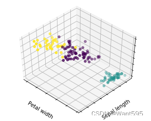
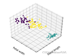
y = iris.targetestimators = {'k_means_iris_3': KMeans(n_clusters=3),'k_means_iris_8': KMeans(n_clusters=8),'k_means_iris_bad_init': KMeans(n_clusters=3, n_init=1,init='random')}fignum = 1
for name, est in estimators.items():fig = plt.figure(fignum, figsize=(4, 3))plt.clf()ax = Axes3D(fig, rect=[0, 0, .95, 1], elev=48, azim=134)plt.cla()est.fit(X)labels = est.labels_ax.scatter(X[:, 3], X[:, 0], X[:, 2], c=labels.astype(np.float))ax.w_xaxis.set_ticklabels([])ax.w_yaxis.set_ticklabels([])ax.w_zaxis.set_ticklabels([])ax.set_xlabel('Petal width')ax.set_ylabel('Sepal length')ax.set_zlabel('Petal length')fignum = fignum + 1# Plot the ground truth
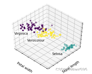
fig = plt.figure(fignum, figsize=(4, 3))
plt.clf()
ax = Axes3D(fig, rect=[0, 0, .95, 1], elev=48, azim=134)plt.cla()for name, label in [('Setosa', 0),('Versicolour', 1),('Virginica', 2)]:ax.text3D(X[y == label, 3].mean(),X[y == label, 0].mean() + 1.5,X[y == label, 2].mean(), name,horizontalalignment='center',bbox=dict(alpha=.5, edgecolor='w', facecolor='w'))
# Reorder the labels to have colors matching the cluster results
y = np.choose(y, [1, 2, 0]).astype(np.float)
ax.scatter(X[:, 3], X[:, 0], X[:, 2], c=y)ax.w_xaxis.set_ticklabels([])
ax.w_yaxis.set_ticklabels([])
ax.w_zaxis.set_ticklabels([])
ax.set_xlabel('Petal width')
ax.set_ylabel('Sepal length')
ax.set_zlabel('Petal length')
plt.show()