Mnist分类任务:
-
网络基本构建与训练方法,常用函数解析
-
torch.nn.functional模块
-
nn.Module模块
-
读取Mnist数据集
- 会自动进行下载
%matplotlib inlinefrom pathlib import Path
import requestsDATA_PATH = Path("data")
PATH = DATA_PATH / "mnist"PATH.mkdir(parents=True, exist_ok=True)URL = "http://deeplearning.net/data/mnist/"
FILENAME = "mnist.pkl.gz"if not (PATH / FILENAME).exists():content = requests.get(URL + FILENAME).content(PATH / FILENAME).open("wb").write(content)import pickle
import gzipwith gzip.open((PATH / FILENAME).as_posix(), "rb") as f:((x_train, y_train), (x_valid, y_valid), _) = pickle.load(f, encoding="latin-1")from matplotlib import pyplot
import numpy as nppyplot.imshow(x_train[0].reshape((28, 28)), cmap="gray")
print(x_train.shape)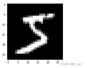
-
\
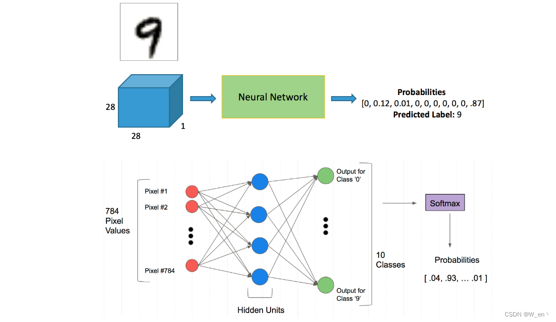
-
注意数据需转换成tensor才能参与后续建模训练
import torchx_train, y_train, x_valid, y_valid = map(torch.tensor, (x_train, y_train, x_valid, y_valid)
)
n, c = x_train.shape
x_train, x_train.shape, y_train.min(), y_train.max()
print(x_train, y_train)
print(x_train.shape)
print(y_train.min(), y_train.max())
torch.nn.functional 很多层和函数在这里都会见到
torch.nn.functional中有很多功能,后续会常用的。那什么时候使用nn.Module,什么时候使用nn.functional呢?一般情况下,如果模型有可学习的参数,最好用nn.Module,其他情况nn.functional相对更简单一些
import torch.nn.functional as Floss_func = F.cross_entropydef model(xb):return xb.mm(weights) + biasbs = 64 xb = x_train[0:bs] # a mini-batch from x yb = y_train[0:bs] weights = torch.randn([784, 10], dtype = torch.float, requires_grad = True) bs = 64 bias = torch.zeros(10, requires_grad=True)print(loss_func(model(xb), yb))创建一个model来更简化代码
- 必须继承nn.Module且在其构造函数中需调用nn.Module的构造函数
- 无需写反向传播函数,nn.Module能够利用autograd自动实现反向传播
- Module中的可学习参数可以通过named_parameters()或者parameters()返回迭代器
from torch import nnclass Mnist_NN(nn.Module):def __init__(self):super().__init__()self.hidden1 = nn.Linear(784, 128)self.hidden2 = nn.Linear(128, 256)self.out = nn.Linear(256, 10)def forward(self, x):x = F.relu(self.hidden1(x))x = F.relu(self.hidden2(x))x = self.out(x)return xnet = Mnist_NN() print(net)
for name, parameter in net.named_parameters():print(name, parameter,parameter.size())hidden1.weight Parameter containing: tensor([[ 0.0018, 0.0218, 0.0036, ..., -0.0286, -0.0166, 0.0089],[-0.0349, 0.0268, 0.0328, ..., 0.0263, 0.0200, -0.0137],[ 0.0061, 0.0060, -0.0351, ..., 0.0130, -0.0085, 0.0073],...,[-0.0231, 0.0195, -0.0205, ..., -0.0207, -0.0103, -0.0223],[-0.0299, 0.0305, 0.0098, ..., 0.0184, -0.0247, -0.0207],[-0.0306, -0.0252, -0.0341, ..., 0.0136, -0.0285, 0.0057]],requires_grad=True) torch.Size([128, 784]) hidden1.bias Parameter containing: tensor([ 0.0072, -0.0269, -0.0320, -0.0162, 0.0102, 0.0189, -0.0118, -0.0063,-0.0277, 0.0349, 0.0267, -0.0035, 0.0127, -0.0152, -0.0070, 0.0228,-0.0029, 0.0049, 0.0072, 0.0002, -0.0356, 0.0097, -0.0003, -0.0223,-0.0028, -0.0120, -0.0060, -0.0063, 0.0237, 0.0142, 0.0044, -0.0005,0.0349, -0.0132, 0.0138, -0.0295, -0.0299, 0.0074, 0.0231, 0.0292,-0.0178, 0.0046, 0.0043, -0.0195, 0.0175, -0.0069, 0.0228, 0.0169,0.0339, 0.0245, -0.0326, -0.0260, -0.0029, 0.0028, 0.0322, -0.0209,-0.0287, 0.0195, 0.0188, 0.0261, 0.0148, -0.0195, -0.0094, -0.0294,-0.0209, -0.0142, 0.0131, 0.0273, 0.0017, 0.0219, 0.0187, 0.0161,0.0203, 0.0332, 0.0225, 0.0154, 0.0169, -0.0346, -0.0114, 0.0277,0.0292, -0.0164, 0.0001, -0.0299, -0.0076, -0.0128, -0.0076, -0.0080,-0.0209, -0.0194, -0.0143, 0.0292, -0.0316, -0.0188, -0.0052, 0.0013,-0.0247, 0.0352, -0.0253, -0.0306, 0.0035, -0.0253, 0.0167, -0.0260,-0.0179, -0.0342, 0.0033, -0.0287, -0.0272, 0.0238, 0.0323, 0.0108,0.0097, 0.0219, 0.0111, 0.0208, -0.0279, 0.0324, -0.0325, -0.0166,-0.0010, -0.0007, 0.0298, 0.0329, 0.0012, -0.0073, -0.0010, 0.0057],requires_grad=True) torch.Size([128]) hidden2.weight Parameter containing: tensor([[-0.0383, -0.0649, 0.0665, ..., -0.0312, 0.0394, -0.0801],[-0.0189, -0.0342, 0.0431, ..., -0.0321, 0.0072, 0.0367],[ 0.0289, 0.0780, 0.0496, ..., 0.0018, -0.0604, -0.0156],...,[-0.0360, 0.0394, -0.0615, ..., 0.0233, -0.0536, -0.0266],[ 0.0416, 0.0082, -0.0345, ..., 0.0808, -0.0308, -0.0403],[-0.0477, 0.0136, -0.0408, ..., 0.0180, -0.0316, -0.0782]],requires_grad=True) torch.Size([256, 128]) hidden2.bias Parameter containing: tensor([-0.0694, -0.0363, -0.0178, 0.0206, -0.0875, -0.0876, -0.0369, -0.0386,0.0642, -0.0738, -0.0017, -0.0243, -0.0054, 0.0757, -0.0254, 0.0050,0.0519, -0.0695, 0.0318, -0.0042, -0.0189, -0.0263, -0.0627, -0.0691,0.0713, -0.0696, -0.0672, 0.0297, 0.0102, 0.0040, 0.0830, 0.0214,0.0714, 0.0327, -0.0582, -0.0354, 0.0621, 0.0475, 0.0490, 0.0331,-0.0111, -0.0469, -0.0695, -0.0062, -0.0432, -0.0132, -0.0856, -0.0219,-0.0185, -0.0517, 0.0017, -0.0788, -0.0403, 0.0039, 0.0544, -0.0496,0.0588, -0.0068, 0.0496, 0.0588, -0.0100, 0.0731, 0.0071, -0.0155,-0.0872, -0.0504, 0.0499, 0.0628, -0.0057, 0.0530, -0.0518, -0.0049,0.0767, 0.0743, 0.0748, -0.0438, 0.0235, -0.0809, 0.0140, -0.0374,0.0615, -0.0177, 0.0061, -0.0013, -0.0138, -0.0750, -0.0550, 0.0732,0.0050, 0.0778, 0.0415, 0.0487, 0.0522, 0.0867, -0.0255, -0.0264,0.0829, 0.0599, 0.0194, 0.0831, -0.0562, 0.0487, -0.0411, 0.0237,0.0347, -0.0194, -0.0560, -0.0562, -0.0076, 0.0459, -0.0477, 0.0345,-0.0575, -0.0005, 0.0174, 0.0855, -0.0257, -0.0279, -0.0348, -0.0114,-0.0823, -0.0075, -0.0524, 0.0331, 0.0387, -0.0575, 0.0068, -0.0590,-0.0101, -0.0880, -0.0375, 0.0033, -0.0172, -0.0641, -0.0797, 0.0407,0.0741, -0.0041, -0.0608, 0.0672, -0.0464, -0.0716, -0.0191, -0.0645,0.0397, 0.0013, 0.0063, 0.0370, 0.0475, -0.0535, 0.0721, -0.0431,0.0053, -0.0568, -0.0228, -0.0260, -0.0784, -0.0148, 0.0229, -0.0095,-0.0040, 0.0025, 0.0781, 0.0140, -0.0561, 0.0384, -0.0011, -0.0366,0.0345, 0.0015, 0.0294, -0.0734, -0.0852, -0.0015, -0.0747, -0.0100,0.0801, -0.0739, 0.0611, 0.0536, 0.0298, -0.0097, 0.0017, -0.0398,0.0076, -0.0759, -0.0293, 0.0344, -0.0463, -0.0270, 0.0447, 0.0814,-0.0193, -0.0559, 0.0160, 0.0216, -0.0346, 0.0316, 0.0881, -0.0652,-0.0169, 0.0117, -0.0107, -0.0754, -0.0231, -0.0291, 0.0210, 0.0427,0.0418, 0.0040, 0.0762, 0.0645, -0.0368, -0.0229, -0.0569, -0.0881,-0.0660, 0.0297, 0.0433, -0.0777, 0.0212, -0.0601, 0.0795, -0.0511,-0.0634, 0.0720, 0.0016, 0.0693, -0.0547, -0.0652, -0.0480, 0.0759,0.0194, -0.0328, -0.0211, -0.0025, -0.0055, -0.0157, 0.0817, 0.0030,0.0310, -0.0735, 0.0160, -0.0368, 0.0528, -0.0675, -0.0083, -0.0427,-0.0872, 0.0699, 0.0795, -0.0738, -0.0639, 0.0350, 0.0114, 0.0303],requires_grad=True) torch.Size([256]) out.weight Parameter containing: tensor([[ 0.0232, -0.0571, 0.0439, ..., -0.0417, -0.0237, 0.0183],[ 0.0210, 0.0607, 0.0277, ..., -0.0015, 0.0571, 0.0502],[ 0.0297, -0.0393, 0.0616, ..., 0.0131, -0.0163, -0.0239],...,[ 0.0416, 0.0309, -0.0441, ..., -0.0493, 0.0284, -0.0230],[ 0.0404, -0.0564, 0.0442, ..., -0.0271, -0.0526, -0.0554],[-0.0404, -0.0049, -0.0256, ..., -0.0262, -0.0130, 0.0057]],requires_grad=True) torch.Size([10, 256]) out.bias Parameter containing: tensor([-0.0536, 0.0007, 0.0227, -0.0072, -0.0168, -0.0125, -0.0207, -0.0558,0.0579, -0.0439], requires_grad=True) torch.Size([10])
-
使用TensorDataset和DataLoader来简化
from torch.utils.data import TensorDataset
from torch.utils.data import DataLoadertrain_ds = TensorDataset(x_train, y_train)
train_dl = DataLoader(train_ds, batch_size=bs, shuffle=True)valid_ds = TensorDataset(x_valid, y_valid)
valid_dl = DataLoader(valid_ds, batch_size=bs * 2)
def get_data(train_ds, valid_ds, bs):return (DataLoader(train_ds, batch_size=bs, shuffle=True),DataLoader(valid_ds, batch_size=bs * 2),) - 一般在训练模型时加上model.train(),这样会正常使用Batch Normalization和 Dropout
- 测试的时候一般选择model.eval(),这样就不会使用Batch Normalization和 Dropout
import numpy as npdef fit(steps, model, loss_func, opt, train_dl, valid_dl):for step in range(steps):model.train()for xb, yb in train_dl:loss_batch(model, loss_func, xb, yb, opt)model.eval()with torch.no_grad():losses, nums = zip(*[loss_batch(model, loss_func, xb, yb) for xb, yb in valid_dl])val_loss = np.sum(np.multiply(losses, nums)) / np.sum(nums)print('当前step:'+str(step), '验证集损失:'+str(val_loss))from torch import optim def get_model():model = Mnist_NN()return model, optim.SGD(model.parameters(), lr=0.001)def loss_batch(model, loss_func, xb, yb, opt=None):loss = loss_func(model(xb), yb)if opt is not None:loss.backward()opt.step()opt.zero_grad()return loss.item(), len(xb)三行搞定!
train_dl, valid_dl = get_data(train_ds, valid_ds, bs)
model, opt = get_model()
fit(25, model, loss_func, opt, train_dl, valid_dl)
当前step:0 验证集损失:2.2796445930480957 当前step:1 验证集损失:2.2440698066711424 当前step:2 验证集损失:2.1889826164245605 当前step:3 验证集损失:2.0985311767578123 当前step:4 验证集损失:1.9517273582458496 当前step:5 验证集损失:1.7341805934906005 当前step:6 验证集损失:1.4719875366210937 当前step:7 验证集损失:1.2273896869659424 当前step:8 验证集损失:1.0362271406173706 当前step:9 验证集损失:0.8963696184158325 当前step:10 验证集损失:0.7927186088562012 当前step:11 验证集损失:0.7141492074012756 当前step:12 验证集损失:0.6529350900650024 当前step:13 验证集损失:0.60417300491333 当前step:14 验证集损失:0.5643046331882476 当前step:15 验证集损失:0.5317994566917419 当前step:16 验证集损失:0.5047958114624024 当前step:17 验证集损失:0.4813900615692139 当前step:18 验证集损失:0.4618900228500366 当前step:19 验证集损失:0.4443243554592133 当前step:20 验证集损失:0.4297310716629028 当前step:21 验证集损失:0.416976597738266 当前step:22 验证集损失:0.406348459148407 当前step:23 验证集损失:0.3963301926612854 当前step:24 验证集损失:0.38733808159828187https://gitee.com/code-wenjiahao/neural-network-practical-classification-and-regression-tasks/tree/master



![[移动通讯]【Carrier Aggregation-3】【5G】](https://img-blog.csdnimg.cn/03095eed827a410182e1a8f74c76bed2.png)

