目录
监督学习算法
线性回归
损失函数
梯度下降
目标函数
更新参数
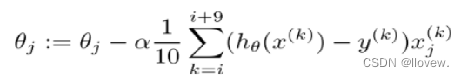
批量梯度下降
随机梯度下降
小批量梯度下降法
数据预处理
特征标准化
正弦函数特征
多项式特征的函数
数据预处理步骤
线性回归代码实现
初始化步骤
实现梯度下降优化模块
损失与预测模块
完整代码
单变量线性回归实例
加载数据并划分数据集
训练线性回归模型得到损失函数图像
测试阶段
多特征回归实例
非线性回归实例
监督学习算法
监督学习算法是一种通过学习输入数据和相应的标签之间的关系来进行预测或分类的方法。
在监督学习中,模型接收带有标签的训练数据,然后通过学习这些数据的模式来进行预测或分类新的未标记数据。
特点:监督学习是使用已知正确答案的示例来训练网络。已知数据和其一一对应的标签,训练一个预测模型,将输入数据映射到标签的过程。
常见应用场景:监督式学习的常见应用场景如分类问题和回归问题。
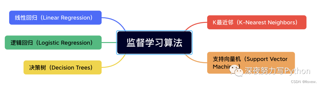
算法举例:常见的有监督机器学习算法包括支持向量机(Support Vector Machine, SVM),朴素贝叶斯(Naive Bayes),逻辑回归(Logistic Regression),K近邻(K-Nearest Neighborhood, KNN),决策树(Decision Tree),随机森林(Random Forest),AdaBoost以及线性判别分析(Linear Discriminant Analysis, LDA)等。深度学习(Deep Learning)也是大多数以监督学习的方式呈现。
线性回归
线性回归是一种用于建立和分析变量之间线性关系的监督学习算法。它主要用于解决回归问题,即预测一个或多个连续数值型输出(因变量)与一个或多个输入特征(自变量)之间的关系。
损失函数
损失函数(Loss Function)是机器学习中用来衡量模型预测结果与实际结果之间差异的一种函数。它是训练模型时所需要最小化或最大化的目标函数,通过调整模型参数,使得损失函数的值达到最小或最大,在模型预测结果与实际结果之间找到最优的拟合程度。
在监督学习中,损失函数通常表示为模型预测结果(例如分类概率或回归值)与实际标签之间的差异。常见的损失函数包括:
1. 均方误差(Mean Squared Error,MSE):计算预测值与真实值之间的平方差的平均值,适用于回归问题。
2. 交叉熵(Cross Entropy):用于分类问题的损失函数,可以衡量模型输出的概率分布与真实标签之间的差异。
3. 对数损失(Logarithmic Loss,或称为逻辑损失,Log Loss):常用于二分类问题的损失函数,衡量模型输出的概率与实际标签之间的负对数似然。
4. Hinge Loss:常用于支持向量机(SVM)中的损失函数,适用于二分类问题进行最大间隔的分类。
5. KL 散度(Kullback-Leibler Divergence):用于衡量两个概率分布之间的差异,常用于生成模型的训练中。
选择合适的损失函数取决于具体的任务和模型类型,不同的损失函数会导致不同的训练效果和模型行为。在实际应用中,通常根据问题的特性和需求选择合适的损失函数来优化模型。
梯度下降
梯度下降法是一种常用的优化算法,用于求解函数的最小值。在机器学习中,我们通常使用梯度下降法来更新模型参数,以最小化损失函数。梯度下降法的基本思想是沿着函数的梯度方向迭代更新参数,直到达到最小值。具体来说,我们首先计算损失函数对于每个参数的梯度,然后按照梯度的反方向更新参数,不断迭代直到收敛。梯度下降法有多种变体,包括批量梯度下降、随机梯度下降和小批量梯度下降等。
- 学习率(步长):对结果会产生巨大的影响,一般小一些
- 如何选择:从小的时候,不行再小
- 批处理数量:32,64,128都可以,很多 时候还得考虑内存和效率

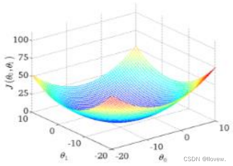
目标函数

寻找山谷的最低点,也就是我们的目标函数终点(什么样的参数能使得目标函数达到极值点)
更新参数
通俗解释下山分几步走呢?
- 找到当前最合适的方向
- 走那么一小步,走快了该”跌倒 ”了
- 按照方向与步伐去更新我们的参数
批量梯度下降
容易得到最优解,但是由于每次考虑所有样本,速度很慢

随机梯度下降
小批量梯度下降法

数据预处理
特征标准化
特征标准化是数据预处理的一种常见方法,用于将不同特征的取值范围进行统一,以便更好地应用于建模和分析过程中。特征标准化函数可以根据不同的需求选择不同的方法进行标准化处理。
- Min-Max标准化:
将特征的取值范围缩放到[0, 1]之间。可以使用sklearn库中的MinMaxScaler函数实现。
from sklearn.preprocessing import MinMaxScalerscaler = MinMaxScaler()
scaled_data = scaler.fit_transform(data)- Z-Score标准化:
通过减去均值并除以标准差,将特征的取值转化为标准正态分布。可以使用sklearn库中的StandardScaler函数实现。
from sklearn.preprocessing import StandardScalerscaler = StandardScaler()
scaled_data = scaler.fit_transform(data)
自定义实现:
# normalize.py
import numpy as np"""首先,函数接受一个名为"features"的参数,这个参数是一个特征矩阵。然后,代码创建了一个名为"features_normalized"的变量,它是输入特征的副本,并转换为浮点型数据。接下来,代码计算了特征矩阵每列的均值,将结果存储在"features_mean"变量中。然后,代码计算了特征矩阵每列的标准差,将结果存储在"features_deviation"变量中。如果特征矩阵的行数大于1,代码会将"features_normalized"减去"features_mean"。这是为了将特征矩阵的每个特征都减去它们的均值。接着,代码将"features_deviation"中值为0的元素替换为1,以避免除以0的错误。最后,代码通过将"features_normalized"除以"features_deviation"来完成归一化操作。函数返回三个值,分别是归一化后的特征矩阵"features_normalized",特征矩阵每列的均值"features_mean"和特征矩阵每列的标准差"features_deviation"。
"""
def normalize(features):# 创建一个与输入特征矩阵相同的副本,并将其转换为浮点型features_normalized = np.copy(features).astype(float)# 计算均值features_mean = np.mean(features, 0)# 计算标准差features_deviation = np.std(features, 0)# 标准化操作if features.shape[0] > 1:features_normalized -= features_mean# 防止除以0,将标准差中为0的元素替换为1,并将特征矩阵除以标准差features_deviation[features_deviation == 0] = 1features_normalized /= features_deviation# 函数返回标准化后的特征矩阵、特征的均值和标准差return features_normalized, features_mean, features_deviation
- Mean归一化:
将特征的取值范围缩放到[-1, 1]之间,使均值为0。可以使用sklearn库中的scale函数实现。
from sklearn.preprocessing import scalescaled_data = scale(data)- 对数归一化:
将特征的取值范围缩放到[0, 1]之间,通过取对数来实现。可以使用numpy库中的log1p函数实现。
import numpy as npscaled_data = np.log1p(data)正弦函数特征
预处理中使用正弦函数特征的原因是因为正弦函数具有周期性和平滑性的特点,可以帮助提取数据中的周期性模式和趋势。在某些情况下,数据可能包含周期性的变化,例如时间序列数据中的季节性变化或周期性信号。通过使用正弦函数特征,可以将这些周期性模式从原始数据中提取出来,从而更好地理解和分析数据。
正弦函数特征还具有平滑性的特点,可以帮助减少数据中的噪声和不规则性。在某些情况下,数据可能受到噪声的干扰或包含不规则的变化。通过使用正弦函数特征,可以对数据进行平滑处理,从而减少噪声的影响并提取出数据中的主要趋势。
总而言之,使用正弦函数特征可以帮助提取数据中的周期性模式和趋势,并减少噪声的影响,从而改善数据的可分析性和预测能力。
# generate_sinusoids.py
import numpy as np"""
生成一组正弦函数的特征。
函数接受两个参数:dataset是一个数据集,sinusoid_degree是正弦函数的阶数。
"""
# 定义了一个名为generate_sinusoids的函数,
# 该函数接受两个参数:dataset(数据集)和sinusoid_degree(正弦函数的最高次数)
def generate_sinusoids(dataset, sinusoid_degree):# 获取数据集的总行数,即数据的示例数。num_examples = dataset.shape[0]"""创建了一个空的numpy数组sinusoids,其形状为(num_examples, 0)。这意味着sinusoids是一个二维数组,其中行数为num_examples,列数为0。由于列数为0,表示该数组没有任何列。这样创建一个空的数组通常是为了在后续的代码中动态地向数组中添加列。通过这种方式,可以根据需要逐步构建数组,而无需提前知道数组的最终大小。"""# 创建一个形状为(num_examples, 0)的空数组sinusoids,用于存储生成的正弦函数特征sinusoids = np.empty((num_examples, 0))for degree in range(1, sinusoid_degree + 1):"""通过一个循环,从1到sinusoid_degree遍历每个阶数。在每个阶数下,函数将输入数据集dataset与当前阶数相乘,并对结果应用正弦函数。生成的正弦函数特征被连接到sinusoids数组中"""# 将每个数据示例乘以degree后计算其正弦值,# 得到一个形状与数据集相同的正弦函数特征数组sinusoid_features。sinusoid_features = np.sin(degree * dataset)"""将两个数组按列连接起来,生成一个新的数组。具体来说,sinusoids和sinusoid_features是两个数组,通过np.concatenate函数将它们按列连接起来,生成一个新的数组"""# 将sinusoid_features按列连接到sinusoids数组中,实现特征的累加。sinusoids = np.concatenate((sinusoids, sinusoid_features), axis=1)# 返回生成的正弦函数特征数组sinusoidsreturn sinusoids
多项式特征的函数
多项式特征函数是一种将原始特征转换为多项式特征的方法。它通过将原始特征的幂次进行组合,生成新的特征矩阵。这种方法可以帮助我们在回归和分类问题中更好地拟合非线性关系。
# generate_polynomials.py
import numpy as np
from .normalize import normalize"""
构建多项式特征的函数。函数名为generate_polynomials,
接受一个数据集dataset、多项式的次数polynomial_degree和一个布尔值normalize_data作为参数。
函数的作用是将输入的数据集生成对应的多项式特征
"""
def generate_polynomials(dataset, polynomial_degree, normalize_data=False):features_split = np.array_split(dataset, 2, axis=1)# 将输入的数据集按列分成两部分,分别赋值给dataset_1和dataset_2dataset_1 = features_split[0]dataset_2 = features_split[1]# 获取dataset_1和dataset_2的行数和列数,# 分别赋值给num_examples_1、num_features_1、num_examples_2和num_features_2(num_examples_1, num_features_1) = dataset_1.shape(num_examples_2, num_features_2) = dataset_2.shape# 判断dataset_1和dataset_2的行数是否相等,如果不相等则抛出ValueError异常if num_examples_1 != num_examples_2:raise ValueError('Can not generate polynomials for two sets with different number of rows')# 判断dataset_1和dataset_2的列数是否都为0,如果是则抛出ValueError异常if num_features_1 == 0 and num_features_2 == 0:raise ValueError('Can not generate polynomials for two sets with no columns')# 判断dataset_1和dataset_2的列数是否有一个为0,如果是则将另一个赋值给它if num_features_1 == 0:dataset_1 = dataset_2elif num_features_2 == 0:dataset_2 = dataset_1# 根据num_features_1和num_features_2的大小确定num_features的值,# 并将dataset_1和dataset_2的列数截取到num_featurenum_features = num_features_1 if num_features_1 < num_examples_2 else num_features_2dataset_1 = dataset_1[:, :num_features]dataset_2 = dataset_2[:, :num_features]# 创建一个空的数组polynomials,用于存储生成的多项式特征polynomials = np.empty((num_examples_1, 0))"""使用两层循环生成多项式特征。外层循环控制多项式的次数,内层循环控制多项式中各项的次数。在每次循环中,根据当前的次数计算多项式特征,并将其与polynomials进行拼接"""for i in range(1, polynomial_degree + 1):for j in range(i + 1):polynomial_feature = (dataset_1 ** (i - j)) * (dataset_2 ** j)polynomials = np.concatenate((polynomials, polynomial_feature), axis=1)# 判断是否对变量polynomials进行归一化处理。如果normalize_data为True,if normalize_data:# 调用normalize函数对polynomials进行归一化处理,并返回处理后的结果polynomials = normalize(polynomials)[0]return polynomials
数据预处理步骤
数据预处理的函数prepare_for_training的目的是对输入的数据进行预处理,为模型训练做准备。它接收一个数据集 `data`,还可以指定一些参数,如 `polynomial_degree`(多项式的次数)、`sinusoid_degree`(正弦函数的次数)和 `normalize_data`(是否对数据进行归一化)。
- 函数会获取数据集的样本数量 `num_examples`,然后对数据进行一份拷贝,存储在 `data_processed` 中。
- 函数会进行数据归一化的处理,如果 `normalize_data` 参数为 `True`,则调用 `normalize` 函数对数据进行归一化处理。归一化的过程会计算数据的均值 `features_mean` 和标准差 `features_deviation`,并将归一化后的数据存储在 `data_normalized` 中。
- 函数会根据参数 `sinusoid_degree` 的值来生成一组正弦函数特征 `sinusoids`,然后将这些特征与归一化后的数据合并,存储在 `data_processed` 中。
- 函数会根据参数 `polynomial_degree` 的值来生成一组多项式特征 `polynomials`,生成过程可能会使用到归一化后的数据,然后将这些特征与之前处理过的数据合并,存储在 `data_processed` 中。
- 函数会在经过处理的数据的左侧添加一列全是1的列向量,以便后续模型训练中的偏置项的计算。
- 函数会返回处理后的数据 `data_processed`,以及归一化过程中计算得到的均值 `features_mean` 和标准差 `features_deviation`。
import numpy as np
from .normalize import normalize
from .generate_sinusoids import generate_sinusoids
from .generate_polynomials import generate_polynomials"""
数据预处理的函数prepare_for_training。
接受一个数据集作为输入,并根据给定的参数进行预处理操作"""
def prepare_for_training(data, polynomial_degree=0, sinusoid_degree=0, normalize_data=True):# 计算样本总数num_examples = data.shape[0]# 创建一个数据副本data_processed,以便在进行预处理操作时不改变原始数据data_processed = np.copy(data)# 预处理features_mean = 0features_deviation = 0data_normalized = data_processed# 如果normalize_data参数为True,则对数据进行归一化处理# 归一化操作将数据的每个特征缩放到0和1之间,# 以消除不同特征之间的量纲差异。同时,记录特征的均值和标准差if normalize_data:(data_normalized,features_mean,features_deviation) = normalize(data_processed)data_processed = data_normalized# 特征变换sinusoidal# 如果sinusoid_degree大于0,则进行正弦特征变换if sinusoid_degree > 0:# generate_sinusoids函数用于生成指定阶数的正弦特征,并将其与原始数据进行连接。sinusoids = generate_sinusoids(data_normalized, sinusoid_degree)data_processed = np.concatenate((data_processed, sinusoids), axis=1)# 特征变换polynomial# 如果polynomial_degree大于0,则进行多项式特征变换if polynomial_degree > 0:# generate_polynomials函数用于生成指定阶数的多项式特征,并将其与原始数据进行连接polynomials = generate_polynomials(data_normalized, polynomial_degree, normalize_data)data_processed = np.concatenate((data_processed, polynomials), axis=1)# 加一列1,将一个全为1的列向量添加到数据的左侧,以便在训练模型时考虑截距data_processed = np.hstack((np.ones((num_examples, 1)), data_processed))# 返回经过预处理后的数据data_processed,以及特征的均值features_mean和标准差features_deviationreturn data_processed, features_mean, features_deviation
线性回归代码实现
初始化步骤
有监督线性回归 传入labels标签 ,normalize_data=True数据进来默认进行预处理操作
def __init__(self,data,labels,polynomial_degree=0, sinusoid_degree=0,normalize_data=True):(data_processed,features_mean,features_deviation) = prepare_for_training(data, polynomial_degree=0, sinusoid_degree=0,normalize_data=True)# 更新data,原始数据经预处理后的数据self.data = data_processedself.labels = labelsself.features_mean = features_meanself.features_deviation = features_deviationself.polynomial_degree = polynomial_degreeself.sinusoid_degree = sinusoid_degreeself.normalize_data = normalize_data# 特征值个数 获取数据的列数num_features = self.data.shape[1]# 构建θ参数矩阵并初始化,θ的个数跟特征的个数一一对应self.theta = np.zeros((num_features,1))
实现梯度下降优化模块
参数更新时算法步骤,每次更新一次
def gradient_step(self,alpha):# 梯度下降算法需要的值:学习率、样本个数、预测值、真实值# 1.样本个数num_examples = self.data.shape[0]# 2.预测值 θ值是不断变化的,传进来变化完之后的θ值,便可得到预测值prediction = LinerRegression.hypothesis(self.data,self.theta) #直接调用# 3.残差计算 预测值减去真实值,真实值为 self.labelsdelta = prediction - self.labels# 4.参数更新 更新θ 进行矩阵计算theta = self.thetatheta = theta - alpha*(1/num_examples)*(np.dot(delta.T,self.data)).T# 5.完成更新self.theta = theta
完成参数更新以及梯度计算
def gradient_descent(self,alpha,num_iterations):# 查看记录损失值变化趋势cost_history = []# 梯度下降核心 迭代for _ in range(num_iterations):# 每迭代一次更新一次self.gradient_step(alpha)# 执行完优化之后将损失值添加到数组中# 定义损失函数计算方法cost_history.append(self.cost_function(self.data,self.labels))# 通过损失函数绘制可视化图return cost_history
帮我们做预测,得到预测值,训练/测试 需要的参数:data、θ
![]()
@staticmethod # 方便调用def hypothesis(self,data,theta):# 预测值计算 真实数据*当前这组参数,predictions = np.dot(data,theta)return predictions损失与预测模块
平方损失函数可从最小二乘法和欧几里得距离角度理解。最小二乘法的原理是,最优拟合曲线应该使所有点到回归直线的距离和最小。损失函数计算:
![]()
def cost_function(self,data,labels):# 获取样本总数num_examples = data.shape[0]# 预测值-真实值delta = LinerRegression.hypothesis(self.data,self.theta) - labels# 定义平方损失函数cost = (1/2)*np.dot(delta.T,delta)# print(cost.shape)return cost[0][0] # 测试集损失函数def get_cost(self,data,labels):# 数据预处理data_processed = prepare_for_training(data, self.polynomial_degree,self.sinusoid_degree, self.normalize_data)[0]return self.cost_function(data_processed,labels)# 测试集预测值def predict(self,data):data_processed = prepare_for_training(data, self.polynomial_degree, self.sinusoid_degree, self.normalize_data)[0]predictions = LinerRegression.hypothesis(data_processed,self.theta)
完整代码
#liner_regression.py
import numpy as np
# 导入预处理模块
from utils.features import prepare_for_trainingclass LinerRegression:# 1.数据预处理# 有监督线性回归 传入labels标签 ,normalize_data=True数据进来默认进行预处理操作def __init__(self,data,labels,polynomial_degree=0, sinusoid_degree=0,normalize_data=True):(data_processed,features_mean,features_deviation) = prepare_for_training(data, polynomial_degree=0, sinusoid_degree=0,normalize_data=True)# 更新data,原始数据经预处理后的数据self.data = data_processedself.labels = labelsself.features_mean = features_meanself.features_deviation = features_deviationself.polynomial_degree = polynomial_degreeself.sinusoid_degree = sinusoid_degreeself.normalize_data = normalize_data# 特征值个数 获取数据的列数num_features = self.data.shape[1]# 构建θ参数矩阵并初始化,θ的个数跟特征的个数一一对应self.theta = np.zeros((num_features,1))# 2.模型训练 参数:学习率α、梯度下降迭代次数def train(self,alpha,num_iterations=500):# 调用梯度下降cost_history = self.gradient_descent(alpha,num_iterations)return self.theta,cost_history# 2-1.梯度下降模块,完成参数更新以及梯度计算def gradient_descent(self,alpha,num_iterations):# 查看记录损失值变化趋势cost_history = []# 梯度下降核心 迭代for _ in range(num_iterations):# 每迭代一次更新一次self.gradient_step(alpha)# 执行完优化之后将损失值添加到数组中# 定义损失函数计算方法cost_history.append(self.cost_function(self.data,self.labels))# 通过损失函数绘制可视化图return cost_history# 2-2.θ参数更新时算法步骤,每次更新一次def gradient_step(self,alpha):# 梯度下降算法需要的值:学习率、样本个数、预测值、真实值# 1.样本个数num_examples = self.data.shape[0]# 2.预测值 θ值是不断变化的,传进来变化完之后的θ值,便可得到预测值prediction = LinerRegression.hypothesis(self.data,self.theta) #直接调用# 3.残差计算 预测值减去真实值,真实值为 self.labelsdelta = prediction - self.labels# 4.参数更新 更新θ  进行矩阵计算theta = self.thetatheta = theta - alpha*(1/num_examples)*(np.dot(delta.T,self.data)).T# 5.完成更新self.theta = theta# 2-3.帮我们做预测,得到预测值,训练/测试 需要的参数:data、θ@staticmethod # 方便调用def hypothesis(self,data,theta):# 预测值计算 真实数据*当前这组参数,predictions = np.dot(data,theta)return predictions# 2-4.损失函数计算def cost_function(self,data,labels):# 获取样本总数num_examples = data.shape[0]# 预测值-真实值delta = LinerRegression.hypothesis(self.data,self.theta) - labels# 定义平方损失函数cost = (1/2)*np.dot(delta.T,delta)# print(cost.shape)return cost[0][0]# 3.测试集损失函数def get_cost(self,data,labels):# 数据预处理data_processed = prepare_for_training(data, self.polynomial_degree,self.sinusoid_degree, self.normalize_data)[0]return self.cost_function(data_processed,labels)# 4.测试集预测值def predict(self,data):data_processed = prepare_for_training(data, self.polynomial_degree, self.sinusoid_degree, self.normalize_data)[0]predictions = LinerRegression.hypothesis(data_processed,self.theta)
单变量线性回归实例
目标:

加载数据并划分数据集
# 单变量线性回归
import numpy as np
import pandas as pd
import matplotlib.pyplot as pltfrom linear_regression import LinerRegression# 读取数据
data = pd.read_csv('../data/world-happiness-report-2017.csv')
# 划分数据集
"""
使用sample()函数从data中随机抽取80%的样本作为训练集,
并将结果赋值给train_data变量。frac = 0.8表示抽取的比例为80%,
random_state = 0表示设置随机种子,保证每次运行代码时得到的随机结果一致
"""
train_data = data.sample(frac = 0.8,random_state = 0)
"""
使用drop()函数删除data中在train_data索引中出现的行,
剩下的行即为测试集,并将结果赋值给test_data变量。
train_data.index表示train_data的索引
"""
test_data = data.drop(train_data.index)# 指定传进来的特征和标签
# 输入特征名字 X
input_param_name = 'Economy..GDP.per.Capita.'
# 输出特征名字 Y
output_param_name = 'Happiness.Score'
# 基于指定列名获取具体数据
x_train = train_data[input_param_name].values
y_train = train_data[output_param_name].valuesx_test = test_data[input_param_name].values
y_test = test_data[output_param_name].values
# 查看数据情况
plt.scatter(x_train,y_train,label="Train data")
plt.scatter(x_test,y_test,label="Test data")
plt.xlabel(input_param_name)
plt.ylabel(output_param_name)
plt.title('Happy')
plt.legend()
plt.show()

训练线性回归模型得到损失函数图像
# 训练模型
# 梯度下降需要传递两个参数 α、num_iterations(迭代次数)
num_iterations = 500
# 定义学习率α
learning_rate = 0.01
"""
参数:
data ----> x_train
labels-----> y_train
polynomial_degree=0(默认)
sinusoid_degree=0(默认)
normalize_data=True(默认)
"""
# 实例化线性回归类
liner_regression= LinerRegression(x_train,y_train)
# 模型训练 参数:学习率α、梯度下降迭代次数,返回θ值和迭代500次所有损失值记录
(theta,cost_history) = liner_regression.train(learning_rate,num_iterations)
print('开始时的损失:',cost_history[0])
print('训练后的损失:',cost_history[-1])# 开始时的损失: 1833.4309980670705
# 训练后的损失: 28.113484781076536# 构建损失函数图像
"""
X:每一次迭代后的损失值
Y:所有的损失值
"""
plt.plot(range(num_iterations),cost_history)
plt.xlabel('Iter')
plt.ylabel('cost')
plt.title('GD')
plt.show()
测试阶段
# 测试阶段
# 测试100个样本
predictions_num = 100
# 通过X预测实际的Y linspace(起始位置,终止位置)
x_predictions = np.linspace(x_train.min(),x_train.max(),predictions_num).reshape(predictions_num,1)
y_predictions = liner_regression.predict(x_predictions)
# 查看数据情况
plt.scatter(x_train,y_train,label="Train data")
plt.scatter(x_test,y_test,label="Test data")
# 回归线
plt.plot(x_predictions,y_predictions,'r',label='Prediction')
plt.xlabel(input_param_name)
plt.ylabel(output_param_name)
plt.title('Happy')
plt.legend()
plt.show()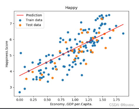
多特征回归实例
# 单变量线性回归
import numpy as np
import pandas as pd
import matplotlib.pyplot as plt
import plotly
import plotly.graph_objs as go
plotly.offline.init_notebook_mode()from linear_regression import LinerRegression# 读取数据
data = pd.read_csv('../data/world-happiness-report-2017.csv')
# 划分数据集
"""
使用sample()函数从data中随机抽取80%的样本作为训练集,
并将结果赋值给train_data变量。frac = 0.8表示抽取的比例为80%,
random_state = 0表示设置随机种子,保证每次运行代码时得到的随机结果一致
"""
train_data = data.sample(frac = 0.8,random_state = 0)
"""
使用drop()函数删除data中在train_data索引中出现的行,
剩下的行即为测试集,并将结果赋值给test_data变量。
train_data.index表示train_data的索引
"""
test_data = data.drop(train_data.index)# 指定传进来的特征和标签
# 输入特征 X1
input_param_name_1 = 'Economy..GDP.per.Capita.'
# 输入特征 X2
input_param_name_2 = 'Freedom'
# 输出特征 Y
output_param_name = 'Happiness.Score'
# 基于指定列名获取具体数据
"""
报错:'numpy.float64' object does not support item assignment
原因:x_train和y_train的值是一维数组[]格式
解决:将x_train和y_train的格式改变为二维数组[[]]
"""
x_train = train_data[[input_param_name_1,input_param_name_2]].values
y_train = train_data[[output_param_name]].valuesx_test = test_data[[input_param_name_1,input_param_name_2]].values
y_test = test_data[[output_param_name]].values
# 查看数据情况
plot_training_trace = go.Scatter3d(x=x_train[:, 0].flatten(),y=x_train[:, 1].flatten(),z=y_train.flatten(),name='Training Set',mode='markers',marker={'size': 10,'opacity': 1,'line': {'color': 'rgb(255, 255, 255)','width': 1},}
)plot_test_trace = go.Scatter3d(x=x_test[:, 0].flatten(),y=x_test[:, 1].flatten(),z=y_test.flatten(),name='Test Set',mode='markers',marker={'size': 10,'opacity': 1,'line': {'color': 'rgb(255, 255, 255)','width': 1},}
)plot_layout = go.Layout(title='Date Sets',scene={'xaxis': {'title': input_param_name_1},'yaxis': {'title': input_param_name_2},'zaxis': {'title': output_param_name}},margin={'l': 0, 'r': 0, 'b': 0, 't': 0}
)plot_data = [plot_training_trace, plot_test_trace]plot_figure = go.Figure(data=plot_data, layout=plot_layout)plotly.offline.plot(plot_figure)# 训练模型
# 梯度下降需要传递两个参数 α、num_iterations(迭代次数)
num_iterations = 500
# 定义学习率α
learning_rate = 0.01
polynomial_degree = 0
sinusoid_degree = 0
"""
参数:
data ----> x_train
labels-----> y_train
polynomial_degree=0(默认)
sinusoid_degree=0(默认)
normalize_data=True(默认)
"""
# 实例化线性回归类
liner_regression= LinerRegression(x_train,y_train,polynomial_degree, sinusoid_degree)
# 模型训练 参数:学习率α、梯度下降迭代次数,返回θ值和迭代500次所有损失值记录
(theta,cost_history) = liner_regression.train(learning_rate,num_iterations)
print('开始时的损失:',cost_history[0])
print('训练后的损失:',cost_history[-1])# 构建损失函数图像
plt.plot(range(num_iterations), cost_history)
plt.xlabel('Iterations')
plt.ylabel('Cost')
plt.title('Gradient Descent Progress')
plt.show()predictions_num = 10x_min = x_train[:, 0].min();
x_max = x_train[:, 0].max();y_min = x_train[:, 1].min();
y_max = x_train[:, 1].max();x_axis = np.linspace(x_min, x_max, predictions_num)
y_axis = np.linspace(y_min, y_max, predictions_num)x_predictions = np.zeros((predictions_num * predictions_num, 1))
y_predictions = np.zeros((predictions_num * predictions_num, 1))x_y_index = 0
for x_index, x_value in enumerate(x_axis):for y_index, y_value in enumerate(y_axis):x_predictions[x_y_index] = x_valuey_predictions[x_y_index] = y_valuex_y_index += 1z_predictions = liner_regression.predict(np.hstack((x_predictions, y_predictions)))plot_predictions_trace = go.Scatter3d(x=x_predictions.flatten(),y=y_predictions.flatten(),z=z_predictions.flatten(),name='Prediction Plane',mode='markers',marker={'size': 1,},opacity=0.8,surfaceaxis=2,
)plot_data = [plot_training_trace, plot_test_trace, plot_predictions_trace]
plot_figure = go.Figure(data=plot_data, layout=plot_layout)
plotly.offline.plot(plot_figure)
非线性回归实例
import numpy as np
import pandas as pd
import matplotlib.pyplot as pltfrom linear_regression import LinerRegressiondata = pd.read_csv('../data/non-linear-regression-x-y.csv')x = data['x'].values.reshape((data.shape[0], 1))
y = data['y'].values.reshape((data.shape[0], 1))data.head(10)plt.plot(x, y)
plt.show()num_iterations = 50000
learning_rate = 0.02
polynomial_degree = 15
sinusoid_degree = 15
normalize_data = True  linear_regression = LinerRegression(x, y, polynomial_degree, sinusoid_degree, normalize_data)(theta, cost_history) = linear_regression.train(learning_rate,num_iterations
)print('开始损失: {:.2f}'.format(cost_history[0]))
print('结束损失: {:.2f}'.format(cost_history[-1]))theta_table = pd.DataFrame({'Model Parameters': theta.flatten()})plt.plot(range(num_iterations), cost_history)
plt.xlabel('Iterations')
plt.ylabel('Cost')
plt.title('Gradient Descent Progress')
plt.show()predictions_num = 1000
x_predictions = np.linspace(x.min(), x.max(), predictions_num).reshape(predictions_num, 1);
y_predictions = linear_regression.predict(x_predictions)plt.scatter(x, y, label='Training Dataset')
plt.plot(x_predictions, y_predictions, 'r', label='Prediction')
plt.show()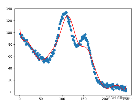


![[python]python实现对jenkins 的任务触发](https://img-blog.csdnimg.cn/7ddd480aac8447b59c56eb11fe4c0067.png)