Reinforcement Learning with Code 【Chapter 10. Actor Critic】
This note records how the author begin to learn RL. Both theoretical understanding and code practice are presented. Many material are referenced such as ZhaoShiyu’s Mathematical Foundation of Reinforcement Learning.
This code refers to Mofan’s reinforcement learning course.
文章目录
- Reinforcement Learning with Code 【Chapter 10. Actor Critic】
- 10.1 The simplest actor-critic algorithm (QAC)
- 10.2 Advantage Actor-Critic (A2C)
- 10.3 Off-policy Actor-Critic
- Reference
10.1 The simplest actor-critic algorithm (QAC)
Recall the idea of policy gradient method is to search for an optimal policy by maximizing a scalar metric J ( θ ) J(\theta) J(θ). The metric has three options, average state value E [ v π ( S ) ] \mathbb{E}[v_\pi(S)] E[vπ(S)], average one step reward E [ r π ( S ) ] \mathbb{E}[r_\pi(S)] E[rπ(S)] or average state value from a specific state s 0 s_0 s0。
According to policy gradient theorem in chapter 9, we are informed that
θ t + 1 = θ t + α ∇ θ J ( θ t ) = θ t + α E S ∼ η , A ∼ π [ ∇ θ ln π ( A ∣ S , θ t ) q π ( S , A ) ] \begin{aligned} \theta_{t+1} & = \theta_t + \alpha \nabla_\theta J(\theta_t) \\ & = \theta_t + \alpha \mathbb{E}_{S\sim\eta, A\sim\pi} [\nabla_\theta \ln \pi(A|S,\theta_t)q_\pi(S,A)] \end{aligned} θt+1=θt+α∇θJ(θt)=θt+αES∼η,A∼π[∇θlnπ(A∣S,θt)qπ(S,A)]
where η \eta η is a distribution of the states. Since the true gradient is unknwon, we can use a stochastic gradient ot approximated it, hence we have
θ t + 1 = θ t + α ∇ θ ln π ( a t ∣ s t , θ t ) q t ( s t , a t ) \theta_{t+1} = \theta_t + \alpha \nabla_\theta \ln\pi(a_t|s_t,\theta_t)q_t(s_t,a_t) θt+1=θt+α∇θlnπ(at∣st,θt)qt(st,at)
- In policy gradient method such as REINFORCE, we use the idea of Monte-Carlo to approximate the true value q t ( s t , a t ) q_t(s_t,a_t) qt(st,at). Where q t ( s t , a t ) q_t(s_t,a_t) qt(st,at) is approximated by an episode return that is q t ( s t , a t ) = ∑ k = t + 1 T γ k − t − 1 r q_t(s_t,a_t)=\sum_{k=t+1}^T \gamma^{k-t-1}r qt(st,at)=∑k=t+1Tγk−t−1r.
- If q t ( s t , a t ) q_t(s_t,a_t) qt(st,at) is estimated by value function approximationg, and the value function is updated using the idea of TD learning. The corresponding algorithms are usually called actor-critic. Therefore, actor-critic methods can be seen as one of the policy gradient method.
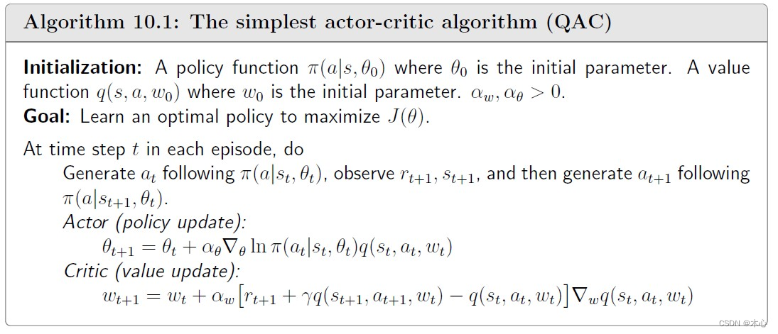
When we use the parameterized value function q ( s , a ; w ) q(s,a;w) q(s,a;w) to approximate the q t ( s t , a t ) q_t(s_t,a_t) qt(st,at), and the value function is updated by the idea of Sarsa of TD learning, the algorithm is called Q actor-critic (QAC). The core idea of QAC is that
QAC: { Actor : θ t + 1 = θ t + α θ ∇ θ ln π ( a t ∣ s t ; θ ) q ( s t , a t ; w t ) Critic : w t + 1 = w t + α w [ r t + 1 + γ q ( s t + 1 , a t + 1 ; w t ) − q ( s t , a t ; w t ) ] ∇ w q ( s t , a t ; w t ) \text{QAC:} \left\{ \begin{aligned} \text{Actor}: \theta_{t+1} & = \theta_t + \alpha_\theta \nabla_\theta \ln\pi(a_t|s_t;\theta) q(s_t,a_t;w_t) \\ \text{Critic}: w_{t+1} & = w_t + \alpha_w [r_{t+1}+\gamma q(s_{t+1},a_{t+1};w_t) - q(s_t,a_t;w_t)]\nabla_w q(s_t,a_t;w_t) \end{aligned} \right. QAC:{Actor:θt+1Critic:wt+1=θt+αθ∇θlnπ(at∣st;θ)q(st,at;wt)=wt+αw[rt+1+γq(st+1,at+1;wt)−q(st,at;wt)]∇wq(st,at;wt)
We use value function approximation to approximate true q value q t ( s t , a t ) q_t(s_t,a_t) qt(st,at). Meanwhile we use the idea of Sarsa to update our value function.
We can write the objective function of the update rule
QAC: { Actor : max θ J ( θ ) = E S ∼ η , A ∼ π [ ln π ( A ∣ S ; θ t ) q ( S , A ; w t ) ] Critic : min w J ( w ) = E S ∼ η , A ∼ π [ ( R + γ q ( S ′ , A ; w t ) − q ( S t , A ; w t ) ) 2 ] \text{QAC:} \left \{ \begin{aligned} \textcolor{red}{\text{Actor}: \max_\theta J(\theta)} & \textcolor{red}{= \mathbb{E}_{S\sim_\eta, A\sim\pi}[\ln\pi(A|S;\theta_t)q(S,A;w_t)]} \\ \textcolor{red}{\text{Critic}: \min_w J(w)} & \textcolor{red}{= \mathbb{E}_{S\sim_\eta, A\sim\pi}[(R + \gamma q(S^\prime,A;w_t) - q(S_t,A;w_t))^2]} \end{aligned} \right. QAC:⎩ ⎨ ⎧Actor:θmaxJ(θ)Critic:wminJ(w)=ES∼η,A∼π[lnπ(A∣S;θt)q(S,A;wt)]=ES∼η,A∼π[(R+γq(S′,A;wt)−q(St,A;wt))2]
Pesudocode
10.2 Advantage Actor-Critic (A2C)
The core idea of A2C is to introduce a baseline to reduce estimation variance. That is
E S ∼ η , A ∼ π [ ∇ θ ln π ( A ∣ S ; θ t ) q π ( S , A ) ] = E S ∼ η , A ∼ π [ ∇ θ ln π ( A ∣ S ; θ t ) ( q π ( S , A ) − b ( S ) ) ] \mathbb{E}_{S\sim\eta,A\sim\pi}[\nabla_\theta \ln \pi(A|S;\theta_t)q_\pi(S,A)] = \mathbb{E}_{S\sim\eta,A\sim\pi}[\nabla_\theta \ln \pi(A|S;\theta_t)(q_\pi(S,A)-b(S))] ES∼η,A∼π[∇θlnπ(A∣S;θt)qπ(S,A)]=ES∼η,A∼π[∇θlnπ(A∣S;θt)(qπ(S,A)−b(S))]
where the additional baseline b ( S ) b(S) b(S) is a scalar function of S S S. Add a baseline doesn’t affect the expectation of the above equation that is
E S ∼ η , A ∼ π [ ∇ θ ln π ( A ∣ S ; θ t ) b ( S ) ] = 0 = ∑ s ∈ S η ( s ) ∑ a ∈ A π ( a ∣ s ; θ t ) ∇ θ ln π ( a ∣ s ; θ t ) b ( s ) = ∑ s ∈ S η ( s ) ∑ a ∈ A ∇ θ π ( a ∣ s ; θ t ) b ( s ) = ∑ s ∈ S η ( s ) b ( s ) ∑ a ∈ A ∇ θ π ( a ∣ s ; θ t ) = ∑ s ∈ S η ( s ) b ( s ) ∇ θ π ∑ a ∈ A ( a ∣ s ; θ t ) = ∑ s ∈ S η ( s ) b ( s ) ∇ θ 1 = 0 \begin{aligned} \mathbb{E}_{S\sim\eta,A\sim\pi}[\nabla_\theta \ln \pi(A|S;\theta_t)b(S)] & = 0 \\ & = \sum_{s\in\mathcal{S}}\eta(s)\sum_{a\in\mathcal{A}}\pi(a|s;\theta_t) \nabla_\theta \ln \pi(a|s;\theta_t)b(s) \\ & = \sum_{s\in\mathcal{S}}\eta(s)\sum_{a\in\mathcal{A}}\nabla_\theta\pi(a|s;\theta_t)b(s) \\ & = \sum_{s\in\mathcal{S}}\eta(s)b(s)\sum_{a\in\mathcal{A}}\nabla_\theta\pi(a|s;\theta_t) \\ & = \sum_{s\in\mathcal{S}}\eta(s)b(s)\nabla_\theta\pi\sum_{a\in\mathcal{A}}(a|s;\theta_t) \\ & = \sum_{s\in\mathcal{S}}\eta(s)b(s)\nabla_\theta1 = 0 \end{aligned} ES∼η,A∼π[∇θlnπ(A∣S;θt)b(S)]=0=s∈S∑η(s)a∈A∑π(a∣s;θt)∇θlnπ(a∣s;θt)b(s)=s∈S∑η(s)a∈A∑∇θπ(a∣s;θt)b(s)=s∈S∑η(s)b(s)a∈A∑∇θπ(a∣s;θt)=s∈S∑η(s)b(s)∇θπa∈A∑(a∣s;θt)=s∈S∑η(s)b(s)∇θ1=0
How to find the optimal baseline? The derivation is omitted. The optimal baseline is
b ∗ ( s ) = E A ∼ π [ ∣ ∣ ∇ θ ln π ( A ∣ s ; θ t ) ∣ ∣ 2 q π ( s , A ) ] E A ∼ π [ ∣ ∣ ∇ θ ln π ( A ∣ s ; θ t ) ∣ ∣ 2 ] b^*(s) = \frac{\mathbb{E}_{A\sim\pi}[||\nabla_\theta \ln\pi(A|s;\theta_t)||^2 q_\pi(s,A)]}{\mathbb{E}_{A\sim\pi}[||\nabla_\theta \ln\pi(A|s;\theta_t)||^2]} b∗(s)=EA∼π[∣∣∇θlnπ(A∣s;θt)∣∣2]EA∼π[∣∣∇θlnπ(A∣s;θt)∣∣2qπ(s,A)]
But its too complex to use in practice. If the weight ∣ ∣ ∇ θ ln π ( A ∣ s ; θ t ) ∣ ∣ 2 ||\nabla_\theta \ln\pi(A|s;\theta_t)||^2 ∣∣∇θlnπ(A∣s;θt)∣∣2 is removed, we can obtain a suboptimal baseline that has a concise expression:
b † ( s ) = E [ q π ( s , A ) ] = v π ( s ) \textcolor{red}{b^\dagger (s) = \mathbb{E}[q_\pi(s,A)] = v_\pi(s)} b†(s)=E[qπ(s,A)]=vπ(s)
The suboptimal baseline is the state value of state s s s.
When b ( s ) = v π ( s ) b(s)=v_\pi(s) b(s)=vπ(s), the gradient-ascent becomes
θ t + 1 = θ t + α E [ ∇ θ ln π ( A ∣ S ; θ t ) [ q π ( S , A ) − v π ( S ) ] ] = θ t + α E [ ∇ θ ln π ( A ∣ S ; θ t ) δ π ( S , A ) ] \begin{aligned} \theta_{t+1} & = \theta_t + \alpha\mathbb{E}[\nabla_\theta \ln\pi(A|S;\theta_t)[q_\pi(S,A)-v_\pi(S)]] \\ & = \theta_t + \alpha\mathbb{E}[\nabla_\theta\ln\pi(A|S;\theta_t) \delta_\pi(S,A)] \end{aligned} θt+1=θt+αE[∇θlnπ(A∣S;θt)[qπ(S,A)−vπ(S)]]=θt+αE[∇θlnπ(A∣S;θt)δπ(S,A)]
Here,
δ π ( S , A ) = q π ( S , A ) − v π ( S ) \textcolor{red}{\delta_\pi(S,A) = q_\pi(S,A) - v_\pi(S)} δπ(S,A)=qπ(S,A)−vπ(S)
is called advantage function, which reflects the advantage of one action over the others. More specifically, note that v π ( s ) = ∑ a ∈ A π ( a ∣ s ) q π ( s , a ) v_\pi(s)=\sum_{a\in\mathcal{A}}\pi(a|s)q_\pi(s,a) vπ(s)=∑a∈Aπ(a∣s)qπ(s,a) is the mean of the action value. If δ π ( s , a ) > 0 \delta_\pi(s,a)>0 δπ(s,a)>0, it means that the corresponding action has a greater value than the mean value.
The stochastic version is
θ t + 1 = θ t + α ∇ θ ln π ( a t ∣ s t ; θ t ) [ q t ( s t , a t ) − v t ( s t ) ] = θ t + α ∇ θ ln π ( a t ∣ s t ; θ t ) δ t ( s t , a t ) \begin{aligned} \theta_{t+1} & = \theta_t + \alpha\nabla_\theta \ln\pi(a_t|s_t;\theta_t)[q_t(s_t,a_t)-v_t(s_t)] \\ & = \theta_t + \alpha\nabla_\theta\ln\pi(a_t|s_t;\theta_t) \delta_t(s_t,a_t) \end{aligned} θt+1=θt+α∇θlnπ(at∣st;θt)[qt(st,at)−vt(st)]=θt+α∇θlnπ(at∣st;θt)δt(st,at)
we need to estimate the true q-value q t ( s t , a t ) q_t(s_t,a_t) qt(st,at). There are many ways:
- If q t ( s t , a t ) q_t(s_t,a_t) qt(st,at) and v t ( s t ) v_t(s_t) vt(st) are estimated by Monte-Carlo learning, the algorithm is called REINFORCE with a baseline.
- If q t ( s t , a t ) q_t(s_t,a_t) qt(st,at) and v t ( s t ) v_t(s_t) vt(st) are estimated by TD learning, the algorithm is usually called advantage actor-critic (A2C).
q t ( s t , a t ) − v t ( s t ) = r t + 1 + γ q t ( s t + 1 , a t + 1 ) − v t ( s t ) ≈ r t + 1 + γ v t ( s t + 1 ) − v t ( s t ) \begin{aligned} q_t(s_t,a_t) - v_t(s_t) & = r_{t+1} +\gamma q_t(s_{t+1},a_{t+1}) - v_t(s_t) \\ & \textcolor{red}{\approx r_{t+1} +\gamma v_t(s_{t+1}) - v_t(s_t)} \end{aligned} qt(st,at)−vt(st)=rt+1+γqt(st+1,at+1)−vt(st)≈rt+1+γvt(st+1)−vt(st)
Hence, we don’t need to maintain two networks to represent v π ( s ) v_\pi(s) vπ(s) and q π ( s , a ) q_\pi(s,a) qπ(s,a). We just need one network to represent v π ( s ) v_\pi(s) vπ(s).
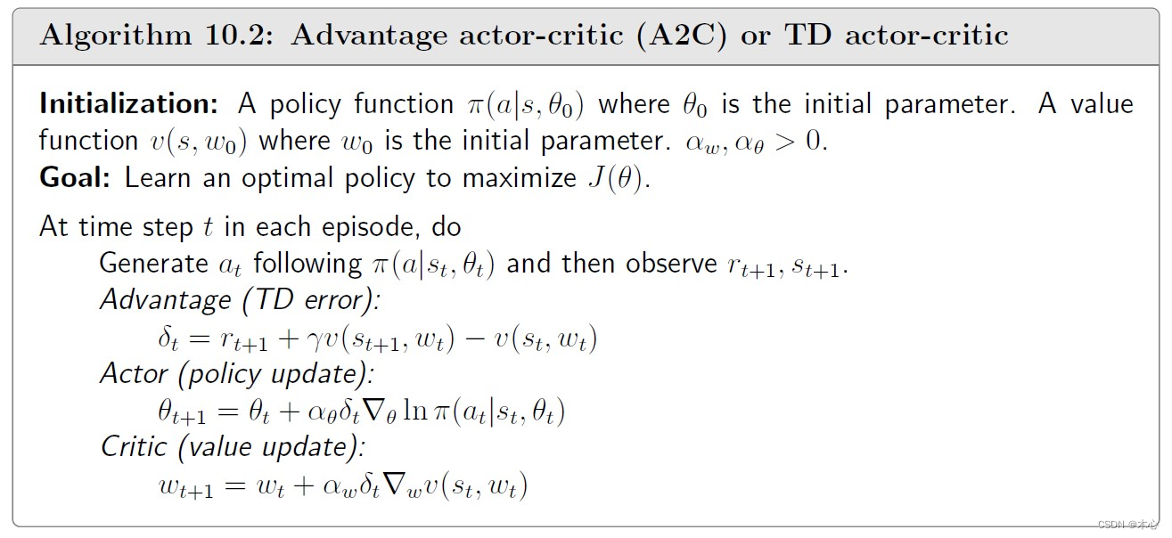
In A2C we use one policy network π ( a ∣ s ; θ ) \pi(a|s;\theta) π(a∣s;θ) and one state value network v ( s ; w ) v(s;w) v(s;w). The core idea of A2C is that
A2C : { Advantage : δ t = r t + 1 + γ v ( s t + 1 ; w t ) − v ( s t ; w t ) Actor : θ t + 1 = θ t + α θ δ t ∇ θ ln π ( a t ∣ s t ; θ ) Critic : w t + 1 = w t + α w δ t ∇ w v ( s t , ; w t ) \text{A2C}: \left \{ \begin{aligned} \text{Advantage}: \delta_t & = r_{t+1} + \gamma v(s_{t+1};w_t) - v(s_t;w_t) \\ \text{Actor}: \theta_{t+1} & = \theta_t + \alpha_\theta \textcolor{blue}{\delta_t}\nabla_\theta \ln\pi(a_t|s_t;\theta) \\ \text{Critic}: w_{t+1} & = w_t + \alpha_w \textcolor{blue}{\delta_t} \nabla_w v(s_t,;w_t) \end{aligned} \right. A2C:⎩ ⎨ ⎧Advantage:δtActor:θt+1Critic:wt+1=rt+1+γv(st+1;wt)−v(st;wt)=θt+αθδt∇θlnπ(at∣st;θ)=wt+αwδt∇wv(st,;wt)
We can write the objective function of the update rule
A2C : { Advantage: Δ ( S ) = R + γ v ( S ′ ; w t ) − v ( S ; w t ) Actor : max θ J ( θ ) = E S ∼ η , A ∼ π [ ln π ( A ∣ S ; θ ) Δ ( S ) ] Critic : min w J ( w ) = E S ∼ η [ ( R + γ v ( S ′ ; w ) − v ( S ; w ) ) 2 ] = E S ∼ η [ Δ ( S ) ] \text{A2C}: \left\{ \begin{aligned} \text{Advantage:} \Delta(S) & = R+\gamma v(S^\prime;w_t) - v(S;w_t) \\ \textcolor{red}{\text{Actor}: \max_\theta J(\theta)} & \textcolor{red}{= \mathbb{E}_{S\sim_\eta, A\sim\pi}[\ln\pi(A|S;\theta)\Delta(S)]} \\ \textcolor{red}{\text{Critic}: \min_w J(w)} & \textcolor{red}{= \mathbb{E}_{S\sim_\eta}[(R + \gamma v(S^\prime;w) - v(S;w))^2]} = \mathbb{E}_{S\sim_\eta}[\Delta(S)] \end{aligned} \right. A2C:⎩ ⎨ ⎧Advantage:Δ(S)Actor:θmaxJ(θ)Critic:wminJ(w)=R+γv(S′;wt)−v(S;wt)=ES∼η,A∼π[lnπ(A∣S;θ)Δ(S)]=ES∼η[(R+γv(S′;w)−v(S;w))2]=ES∼η[Δ(S)]
Pesudocode
10.3 Off-policy Actor-Critic
Importance Sampling
The key technique to convert the AC algorithm to off-policy is importance sampling. Consider a random variable X ∈ X X\in\mathcal{X} X∈X. Suppose that p 0 ( X ) p_0(X) p0(X) is a probability distribution. Our goal is to estimate E X ∼ p 0 [ X ] \mathbb{E}_{X\sim p_0}[X] EX∼p0[X]. We also known the p 1 ( X ) p_1(X) p1(X) is a probability distribution of X X X. How can we use the probability p 1 ( X ) p_1(X) p1(X) to sample data to estimate E X ∼ p 0 [ X ] \mathbb{E}_{X\sim p_0}[X] EX∼p0[X]. The technique is importance sampling. Suppose we have some i.i.d. samples { x i } i = 1 n \{x_i\}^n_{i=1} {xi}i=1n generated by distribution p 1 ( X ) p_1(X) p1(X).
E X ∼ p 0 [ X ] = ∑ x ∈ X p 0 ( x ) x = ∑ x ∈ X p 1 ( x ) p 0 ( x ) p 1 ( x ) x ⏟ f ( x ) = E X ∼ p 1 [ f ( X ) ] E X ∼ p 0 [ X ] = E X ∼ p 1 [ f ( X ) ] ≈ f ˉ = 1 n ∑ i = 1 n f ( x i ) = 1 n ∑ i = 1 n p 0 ( x i ) p 1 ( x i ) ⏟ importance weight x i \mathbb{E}_{X\sim p_0}[X] = \sum_{x\in\mathcal{X}}p_0(x)x = \sum_{x\in\mathcal{X}}p_1(x)\underbrace{\frac{p_0(x)}{p_1(x)}x}_{f(x)} = \mathbb{E}_{X\sim p_1}[f(X)] \\ \mathbb{E}_{X\sim p_0}[X] = \mathbb{E}_{X\sim p_1}[f(X)] \approx \bar{f} = \frac{1}{n} \sum^n_{i=1}f(x_i) = \frac{1}{n} \sum^n_{i=1} \underbrace{\frac{p_0(x_i)}{p_1(x_i)}}_{\text{importance weight}}x_i EX∼p0[X]=x∈X∑p0(x)x=x∈X∑p1(x)f(x) p1(x)p0(x)x=EX∼p1[f(X)]EX∼p0[X]=EX∼p1[f(X)]≈fˉ=n1i=1∑nf(xi)=n1i=1∑nimportance weight p1(xi)p0(xi)xi
An Example
Consider X ∈ X = + 1 , − 1 X\in\mathcal{X}={+1,-1} X∈X=+1,−1 Suppose the p 0 p_0 p0 is a probability distribution satisfying
p 0 ( X = + 1 ) = 0.5 , p 0 ( X = − 1 ) = 0.5 p_0(X=+1)=0.5, p_0(X=-1)=0.5 p0(X=+1)=0.5,p0(X=−1)=0.5
The expectaton of X X X over p 0 p_0 p0 is
E X ∼ p 0 [ X ] = ( + 1 ) × 0.5 + ( − 1 ) × 0.5 = 0 \mathbb{E}_{X\sim p_0}[X] = (+1)\times 0.5 + (-1) \times 0.5 = 0 EX∼p0[X]=(+1)×0.5+(−1)×0.5=0
Suppose p 1 p_1 p1 is a probability distribution satisfying
p 0 ( X = + 1 ) = 0.8 , p 0 ( X = − 1 ) = 0.2 p_0(X=+1)=0.8, p_0(X=-1)=0.2 p0(X=+1)=0.8,p0(X=−1)=0.2
The expectaton of X X X over p 0 p_0 p0 is
E X ∼ p 1 [ X ] = ( + 1 ) × 0.8 + ( − 1 ) × 0.2 = 0.6 \mathbb{E}_{X\sim p_1}[X] = (+1)\times 0.8 + (-1) \times 0.2 = 0.6 EX∼p1[X]=(+1)×0.8+(−1)×0.2=0.6
We can use the importance samping techique to sample data under distribution p 1 p_1 p1 to compute E X ∼ p 0 [ X ] \mathbb{E}_{X\sim p_0}[X] EX∼p0[X]
E X ∼ p 0 [ X ] = 1 n ∑ i = 1 n p 0 ( x i ) p 1 ( x i ) x i \mathbb{E}_{X\sim p_0}[X] = \frac{1}{n}\sum_{i=1}^n \frac{p_0(x_i)}{p_1(x_i)}x_i EX∼p0[X]=n1i=1∑np1(xi)p0(xi)xi
import numpy as np
import matplotlib.pyplot as plt
# reproducible
np.random.seed(0)# 定义元素和对应的概率
elements = [1, -1]
probs1 = [0.5, 0.5]
probs2 = [0.8, 0.2]# 重要性采样 importance sample
sample_times = 300
sample_list = []
i_sample_list = []
average_list = []
importance_list = []
for i in range(sample_times):sample = np.random.choice(elements, p=probs2)sample_list.append(sample)average_list.append(np.mean(sample_list))if sample == elements[0]:i_sample_list.append(probs1[0] / probs2[0] * sample)elif sample == elements[1]:i_sample_list.append(probs1[1] / probs2[1] * sample)importance_list.append(np.mean(i_sample_list))plt.plot(range(len(sample_list)), sample_list, 'o', markerfacecolor='none', label='sample data')
plt.plot(range(len(average_list)), average_list, 'b--', label='average')
plt.plot(range(len(importance_list)), importance_list, 'g--', label='importance sampling')
plt.axhline(y=0.6, color='r', linestyle='--')
plt.axhline(y=0, color='r', linestyle='--')
plt.ylim(-1.5, 2.5) # 限制y轴显示范围
plt.xlim(0,sample_times) # 限制x轴显示范围
plt.legend(loc='upper right')
plt.show()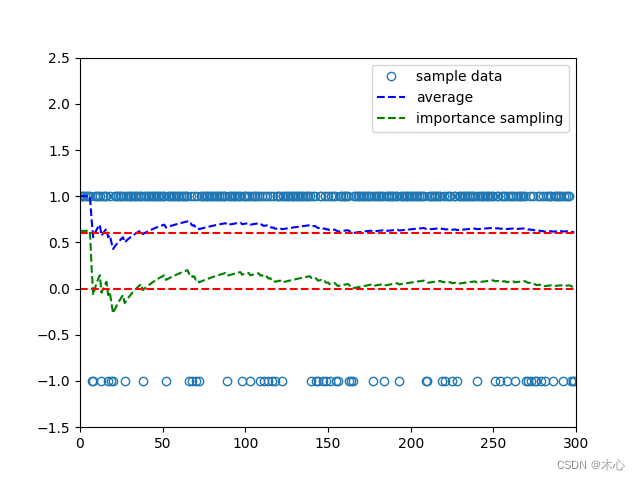
Off-policy policy gradient theorem
With importance sampling, we are ready to present the off-policy gradient theorem. Suppose that the β \beta β is a behavior policy. Our goal is to use the samples generated by behavoir policy β \beta β to learn a target policy π \pi π that can maximize the following metric
max θ J ( θ ) = E S ∼ d β [ v π ( S ) ] \max_\theta J(\theta) = \mathbb{E}_{S\sim d_\beta}[v_\pi(S)] θmaxJ(θ)=ES∼dβ[vπ(S)]
Theorem 10.1 (Stochastic off-policy policy gradient theorem). In the discounted case where γ ∈ ( 0 , 1 ) \gamma\in(0,1) γ∈(0,1), the gradient of J ( θ ) J(\theta) J(θ) is
∇ θ J ( θ ) = E S ∼ ρ , A ∼ β [ π ( A ∣ S ; θ ) β ( A ∣ S ) ⏟ importance weight ∇ θ ln π ( A ∣ S ; θ ) q π ( S , A ) ] \textcolor{red}{\nabla_\theta J(\theta) = \mathbb{E}_{S\sim\rho, A\sim\beta}\Big[\underbrace{\frac{\pi(A|S;\theta)}{\beta(A|S)}}_{\text{importance weight}} \nabla_\theta \ln \pi(A|S;\theta) q_\pi(S,A) \Big]} ∇θJ(θ)=ES∼ρ,A∼β[importance weight β(A∣S)π(A∣S;θ)∇θlnπ(A∣S;θ)qπ(S,A)]
where the state distribution ρ \rho ρ is
ρ ( s ) ≜ ∑ s ′ ∈ S d β ( s ′ ) Pr π ( s ∣ s ′ ) \rho(s) \triangleq \sum_{s^\prime\in\mathcal{S}} d_\beta(s^\prime) \Pr_\pi(s|s^\prime) ρ(s)≜s′∈S∑dβ(s′)πPr(s∣s′)
where Pr π ( s ∣ s ′ ) = ∑ k = 0 ∞ γ k [ P π k ] s ′ , s = [ ( I − γ P π ) − 1 ] s ′ , s \Pr_\pi(s|s^\prime)=\sum_{k=0}^\infty \gamma^k[P^k_\pi]_{s^\prime,s}=[(I-\gamma P_\pi)^{-1}]_{s^\prime,s} Prπ(s∣s′)=∑k=0∞γk[Pπk]s′,s=[(I−γPπ)−1]s′,s is the discounted total probability of transitioning from s ′ s^\prime s′ to s s s under policy π \pi π.
The off-policy policy gradient is invariant to any additional baseline b ( s ) b(s) b(s). In particular, we have
∇ θ J ( θ ) = E S ∼ ρ , A ∼ β [ π ( A ∣ S ; θ ) β ( A ∣ S ) ∇ θ ln π ( A ∣ S ; θ ) ( q π ( S , A ) − b ( S ) ) ] \nabla_\theta J(\theta) = \mathbb{E}_{S\sim\rho, A\sim\beta}\Big[\frac{\pi(A|S;\theta)}{\beta(A|S)} \nabla_\theta \ln \pi(A|S;\theta) \big( q_\pi(S,A) - b(S) \big) \Big] ∇θJ(θ)=ES∼ρ,A∼β[β(A∣S)π(A∣S;θ)∇θlnπ(A∣S;θ)(qπ(S,A)−b(S))]
when we take the state value as the baseline v π ( S ) = b ( S ) v_\pi(S)=b(S) vπ(S)=b(S), there comes the advantage function.
δ π ( S , A ) = q π ( S , A ) − v π ( S ) \delta_\pi(S,A) = q_\pi(S,A) - v_\pi(S) δπ(S,A)=qπ(S,A)−vπ(S)
The corresponding stochastic gradient-ascent algorithm is
θ t + 1 = θ t + α θ π ( a t ∣ s t ; θ ) β ( a t ∣ s t ) ∇ θ ln π ( a t ∣ s t ; θ t ) ( q t ( s t , a t ) − v t ( s t ) ) \theta_{t+1} = \theta_t + \alpha_\theta \frac{\pi(a_t|s_t;\theta)}{\beta(a_t|s_t)} \nabla_\theta \ln\pi(a_t|s_t;\theta_t)(q_t(s_t,a_t)-v_t(s_t)) θt+1=θt+αθβ(at∣st)π(at∣st;θ)∇θlnπ(at∣st;θt)(qt(st,at)−vt(st))
The advantage function can be replaced by the TD error. That is
q t ( s t , a t ) − v t ( s t ) ≈ r t + 1 + γ v t ( s t + 1 ) − v t ( s t ) ≜ δ t ( s t , a t ) q_t(s_t,a_t)-v_t(s_t) \approx r_{t+1} + \gamma v_t(s_{t+1}) - v_t(s_t) \triangleq \delta_t(s_t,a_t) qt(st,at)−vt(st)≈rt+1+γvt(st+1)−vt(st)≜δt(st,at)
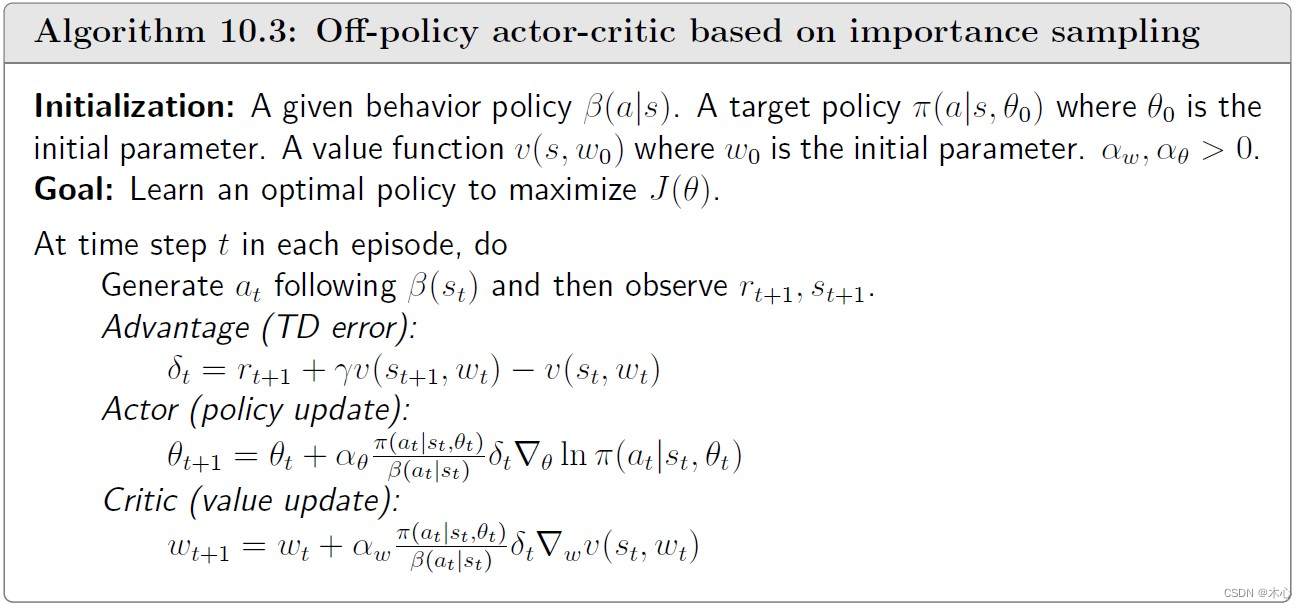
In off-policy A2C we use the behavior policy β \beta β to obtain samples, to learn a policy network π ( a ∣ s ; θ ) \pi(a|s;\theta) π(a∣s;θ), and one value network v ( s ; w ) v(s;w) v(s;w). The core idea of off-policy A2C is
off-policy A2C : { Behavior policy: S ∼ β Advantage : δ t = r t + 1 + γ v ( s t + 1 ; w t ) − v ( s t ; w t ) Actor : θ t + 1 = θ t + α θ π ( a t ∣ s t ; θ ) β ( a t ∣ s t ) δ t ∇ θ ln π ( a t ∣ s t ; θ ) Critic : w t + 1 = w t + α w π ( a t ∣ s t ; θ ) β ( a t ∣ s t ) δ t ∇ w v ( s t , ; w t ) \text{off-policy A2C}: \left \{ \begin{aligned} \text{Behavior policy:} S & \sim\beta \\ \text{Advantage}: \delta_t & = r_{t+1} + \gamma v(s_{t+1};w_t) - v(s_t;w_t) \\ \text{Actor}: \theta_{t+1} & = \theta_t + \alpha_\theta \frac{\pi(a_t|s_t;\theta)}{\beta(a_t|s_t)} \delta_t\nabla_\theta \ln\pi(a_t|s_t;\theta) \\ \text{Critic}: w_{t+1} & = w_t + \alpha_w \frac{\pi(a_t|s_t;\theta)}{\beta(a_t|s_t)}\delta_t \nabla_w v(s_t,;w_t) \end{aligned} \right. off-policy A2C:⎩ ⎨ ⎧Behavior policy:SAdvantage:δtActor:θt+1Critic:wt+1∼β=rt+1+γv(st+1;wt)−v(st;wt)=θt+αθβ(at∣st)π(at∣st;θ)δt∇θlnπ(at∣st;θ)=wt+αwβ(at∣st)π(at∣st;θ)δt∇wv(st,;wt)
We rewrite the objective function of the update rule
off-policy A2C : { Behavior policy: S ∼ β Advantage : Δ ( S ) = R + γ v ( S ′ ; w ) − v ( S ; w ) Actor : max θ J ( θ ) = E S ∼ ρ , A ∼ β [ π ( A ∣ S ; θ ) β ( A ∣ S ) Δ ( S ) ln π ( A ∣ S ; θ ) ] Critic : min w J ( w ) = E S ∼ ρ [ ( R + γ v ( S ′ ; w t ) − v ( S t ; w t ) ) 2 ] = E S ∼ η [ Δ ( S ) ] \text{off-policy A2C}: \left \{ \begin{aligned} \text{Behavior policy:} S & \sim\beta \\ \text{Advantage}: \Delta(S) & = R + \gamma v(S^\prime;w) - v(S;w) \\ \text{Actor}: \max_\theta J(\theta) & = \mathbb{E}_{S\sim\rho,A\sim\beta}[\frac{\pi(A|S;\theta)}{\beta(A|S)}\Delta(S) \ln\pi(A|S;\theta)] \\ \text{Critic}: \min_w J(w) & = \mathbb{E}_{S\sim\rho}[(R + \gamma v(S^\prime;w_t) - v(S_t;w_t))^2] = \mathbb{E}_{S\sim_\eta}[\Delta(S)] \end{aligned} \right. off-policy A2C:⎩ ⎨ ⎧Behavior policy:SAdvantage:Δ(S)Actor:θmaxJ(θ)Critic:wminJ(w)∼β=R+γv(S′;w)−v(S;w)=ES∼ρ,A∼β[β(A∣S)π(A∣S;θ)Δ(S)lnπ(A∣S;θ)]=ES∼ρ[(R+γv(S′;wt)−v(St;wt))2]=ES∼η[Δ(S)]
Pesudocode
Reference
赵世钰老师的课程