DQNs【Vanilla DQN & Double DQN & Dueling DQN】

​ 在 Reinforcement Learning with Code 【Code 1. Tabular Q-learning】中讲解的 Q-learning 算法中，我们以矩阵的方式建立了一张存储每个状态下所有动作 $Q$值的表格。表格中的每一个动作价值 $Q(s,a)$表示在状态 $s$下选择动作然后继续遵循某一策略预期能够得到的期望回报。然而，这种用表格存储动作价值的做法只在环境的状态和动作都是离散的，并且空间都比较小的情况下适用。当状态或者动作数量非常大的时候，这种做法就不适用了。例如，当状态是一张 RGB 图像时，假设图像大小是 $210\times 160\times 3$，此时一共有 $256^{(210\times 160\times 3)}$种状态，在计算机中存储这个数量级的值表格是不现实的。更甚者，当状态或者动作连续的时候，就有无限个状态动作对，我们更加无法使用这种表格形式来记录各个状态动作对的 $Q$值。

​ 对于这种情况，我们需要用函数拟合的方法来估计值$Q$，即将这个复杂的$Q$值表格视作数据，使用一个参数化的函数$Q_{\theta }$来拟合这些数据。很显然，这种函数拟合的方法存在一定的精度损失，因此被称为近似方法。我们今天要介绍的 DQN 算法便可以用来解决连续状态下离散动作的问题。

1. DQN及其变种介绍

1.1 Vanilla DQN

Vanilla DQN便是最基本的DQN算法，在Q-learning中需要优化的目标函数为
$$\underset{\theta }{\min }J(\theta )=\mathbb{E}\left[\right(R+\gamma \underset{a}{\max }Q(S^{\prime },a;\theta )-Q(S,A;\theta )\left)\right]$$
在Q-learning中的TD target是 $Y_t^Q=R_{t+1}+\gamma {\max }_{a}Q(S_{t+1},a;{\theta }_t)$，若直接更新上述网络需要考虑很复杂的时许问题，在DQN使用了两个网络来简化这一过程。

Vallina DQN使用两个技巧：

• Experience Replay，维护了一个经验池，将智能体与环境交互的experience $(s,a,r,s^{\prime },\text{done})$存储进经验池中，然后再从维护的经验池中取出experience来进行训练，这样做有两个好处，第一，因为我们所解决的问题是被建模成Markov Decision Process（MDP）。在 MDP 中交互采样得到的数据本身不满足独立假设，因为这一时刻的状态和上一时刻的状态有关。非独立同分布的数据对训练神经网络有很大的影响，会使神经网络拟合到最近训练的数据上。采用经验回放可以打破样本之间的相关性，让其满足独立假设。第二，提高样本效率。每一个样本可以被使用多次，十分适合深度神经网络的梯度学习。

• Two Networks， Vanilla DQN为了解决训练中的更新时序问题，在未引入两套网络之前，是希望网络的参数$\theta$能够跟踪$Y_t^Q=R_{t+1}+\gamma {\max }_{a}Q(S_{t+1},a;{\theta }_t)$，其中$Y_t^Q$被称为TD target。引入了两套网络后，分记为训练网络和目标网路，网络参数分别用$\theta$和${\theta }^{-}$来表示，Vanilla DQN的最终目的是让目标网络${\theta }^{-}$的输出能够逼近
  $$Y_t^{DQN}=R_{t+1}+\gamma \underset{a}{\max }Q(S_{t+1},a;{\theta }^{-})$$
  所以这样之后，待优化的目标函数变成了
  $$\underset{\theta }{\min }J(\theta )=\mathbb{E}\left[\right(R+\gamma \underset{a}{\max }Q(S^{\prime },a;{\theta }^{-})-Q(S,A;\theta )\left)\right]$$
  我们使用这个目标函数来作为Vallina DQN需要优化的损失函数来更新训练网络参数$\theta$，然后每隔$\tau$代，将训练网络参数$\theta$拷贝给目标网络${\theta }^{-}$。

1.2 Double DQN

Double DQN的提出是用于解决Vallina DQN在实际应用中对Q值估计过高的问题（overestimation）。Vallina DQN的优化TD target是
$$Y_t^{DQN}=R_{t+1}+\gamma \underset{a}{\max }Q(S_{t+1},a;{\theta }^{-})$$
其中${\max }_{a}Q(S_{t+1},a;{\theta }^{-})$是由目标网络的参数${\theta }^{-}$计算而来的，那么我们可以获得最优的动作$a^{\ast }=\arg {\max }_{a}Q(S_{t+1},a;{\theta }^{-})$，将最优的动作带回，则我们可以将上式进行改写成
$$Y_t^{DQN}=R_{t+1}+\gamma Q(S_{t+1},\arg \underset{a}{\max }Q(S_{t+1},a;{\theta }^{-});{\theta }^{-})$$
换句话说$\max$操作其实可以分为两部分，首先选取状态$S_{t+1}$下的最优的动作$a^{\ast }=\arg {\max }_{a}Q(S_{t+1},a;{\theta }^{-})$接着计算该动作对于的价值$Q(S_{t+1},a^{\ast };{\theta }^{-})$。但是当这两个部分都采用同一套Q网络来进行训练时，每次计算得到的都是神经网络中当前估计的所有动作价值中最大值。考虑到通过神经网络估计的Q值本身在某些时刻也会产生正向或负向的误差，在DQN的更新方式下神经网络会将正向误差进行累积。

为了解决这一问题，Double DQN提出了利用两个独立的网络估算${\max }_a{Q}^{\ast }(S_{t+1},A_{t+1})$。具体的做法是将原有的${\max }_{a}Q(S_{t+1},a;{\theta }^{-})$更改为$Q(S_{t+1},\arg {\max }_{a}Q(S_{t+1},a;\theta ),{\theta }^{-})$。即利用一套训练网络$\theta$来选取价值最大的动作，用目标神经网络${\theta }^{-}$来计算该动作的价值。这样，即使其中一套神经网络的某个动作存在比较严重的过高估计问题，由于另一套神经网络的存在，这个动作最终使得Q值不会被过高估计。则我们可以将Double DQN的TD target写作
$$Y_t^{DDQN}=R_{t+1}+\gamma Q(S_{t+1},\arg \underset{a}{\max }Q(S_{t+1},a;\theta );{\theta }^{-})$$
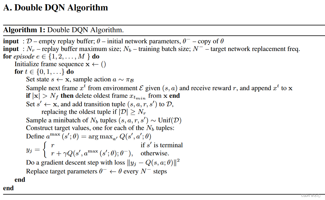
Pesudocode

1.3 Dueling DQN

Dueling DQN是Vanilla DQN的一种变种算法，它在传统Vanilla DQN的基础上只进行了微小的改动，却大幅提升了DQN的表现能力。具体来说就是Dueling DQN并未直接来估计Q值函数，而是通过估计V状态价值函数和A优势函数来间接获得Q值函数。Dueling DQN非常创新地引入了优势函数的概念（Advantage function），在介绍优势函数之前，我们先回顾一下动作价值函数Q和状态价值函数V的定义：
$$\begin{gathered} Q^{\pi }(s,a)=\mathbb{E}[R_t|s_t=s,a_t=a,\pi ] \\ {V}^{\pi }(s,a)={\mathbb{E}}_{a\sim \pi }[Q^{\pi }(s,a)] \end{gathered}$$
优势函数（Advantage function）被定义为
$$A^{\pi }(s,a)=Q^{\pi }(s,a)-V^{\pi }(s)$$
我们对优势函数取服从$a\sim \pi$的期望，则有
$$A^{\pi }(s,a)={\mathbb{E}}_{a\sim \pi }[Q^{\pi }(s,a)]-{\mathbb{E}}_{a\sim \pi }[Q^{\pi }(s,a)]=0$$
直观上来理解，状态价值函数V衡量的是处于状态$s$的好坏程度，然而，Q函数衡量的是在此状态$s$下选择特定操作的价值，优势函数A是从Q函数中减去状态值V，来获得每个动作重要性的相对程度。对于确定性的策略$\pi$，最优的动作可以表示为
$$a^{\ast }=\arg \underset{a^{\prime }\in \mathcal{A}}{\max }Q(s,a^{\prime })$$
又因为策略是确定性的，那么则有
$$Q(s,a^{\ast })=V(s)$$
那么对于最优动作$a^{\ast }$的优势函数则有
$$A(s,a^{\ast })=0$$
接下来介绍下在网络结构上的创新，在Dueling DQN中为了实现上述的势函数网络结构也发生了变化，

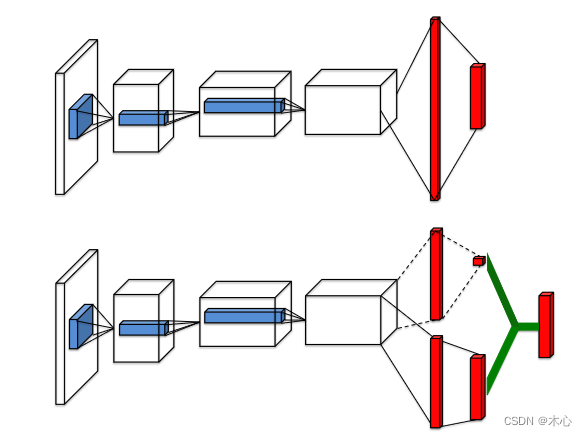
在图中，位于上方的网络结构是DQN的结构，位于下方的网络结构是Dueling DQN的结构。Dueling网络有两个流来分别估计状态值V（scalar）和每个动作的优势A（vector）；绿色输出模块实现等式$A^{\pi }(s,a)=Q^{\pi }(s,a)-V^{\pi }(s)$以将它们结合起来。结合上述的网络结构，我们将网络结构的参数加上，来重写优势函数A的表达式
$$\begin{array}{rl}A(s,a;\theta ,\alpha )& =Q(s,a;\theta ,\alpha ,\beta )-V(s;\theta ,\beta )\\ Q(s,a;\theta ,\alpha ,\beta )& =A(s,a;\theta ,\alpha )+V(s;\theta ,\beta )\end{array}$$
其中，$\theta$代表了前面共享网络结构的参数，$\alpha ,\beta$分别代表两个流各自的网络结构参数。但是上述式子中存在着对于V值，A值的唯一性不确定的问题，为了解决这一问题，我们对于同样的Q值加上任意大小的常数C，再将所有A值减去C，这样得到的Q值仍然不变，这就导致了训练的不稳定性，为了解决这一问题，Dueling DQN强制将最优动作的优质函数输出置为0，即
$$Q(s,a;\theta ,\alpha ,\beta )=V(s;\theta ,\beta )+(A(s,a;\theta ,\alpha )-\underset{a^{\prime }\in \mathcal{A}}{\max }A(s,a^{\prime };\theta ,\alpha ))$$
根据之前的分析我们知道，对于最优的动作$a^{\ast }$，优势函数的值为0，即$A(s,a^{\ast })=0$，对于最优的动作$a^{\ast }$
$$\begin{array}{rl}{a}^{\ast }& =\arg \underset{a^{\prime }\in \mathcal{A}}{\max }Q(s,a^{\prime };\theta ,\alpha ,\beta )\\ & =\arg \underset{a^{\prime }\in \mathcal{A}}{\max }[A(s,a;\theta ,\alpha )+V(s;\theta ,\beta )]\\ & =\arg \underset{a^{\prime }\in \mathcal{A}}{\max }A(s,a;\theta ,\alpha )\end{array}$$
再将最优动作$a^{\ast }$代回上式中，则有
$$Q(s,a^{\ast };\theta ,\alpha ,\beta )=V(s;\theta ,\beta )$$
因此这样就成功实现了解耦，一个流$V(s;\theta ,\beta )$提供状态价值的估计，另一个流$A(s,a;\theta ,\alpha )$实现优势值的估计。

在实际中，我们常用平均（average）操作来替换最大值（max）操作，这样更具稳定性，如下
$$Q(s,a;\theta ,\alpha ,\beta )=V(s;\theta ,\beta )+(A(s,a;\theta ,\alpha )-\frac{1}{|\mathcal{A}|}A(s,a^{\prime };\theta ,\alpha ))$$
将上述Q值函数来计算Vanilla DQN中的TD target就能得到Dueling DQN的TD target，再按照Vanilla DQN剩下的方法来进行更新，我们就得到了Dueling DQN的完整算法。
$$Y_t^{\text{DuelingDQN}}=R_{t+1}+\gamma \underset{a}{\max }Q(S_{t+1},a;\theta ,\alpha ,\beta )$$
其中$Q(S_{t+1},a;\theta ,\alpha ,\beta )$可以替换成average操作产生的结果，那么完整的TD target就成了
$$Y_t^{\text{DuelingDQN}}=R_{t+1}+\gamma V(s;\theta ,\beta )+\gamma \underset{a}{\max }(A(s,a;\theta ,\alpha )-\frac{1}{|\mathcal{A}|}A(s,a^{\prime };\theta ,\alpha ))$$
其中$Q(S_{t+1},a;\theta ,\alpha ,\beta )$也可以替换成max操作产生的记过，那么完整的TD target就成了
$$Y_t^{\text{DuelingDQN}}=R_{t+1}+\gamma V(s;\theta ,\beta )+\gamma \underset{a}{\max }(A(s,a;\theta ,\alpha )-\underset{a^{\prime }\in \mathcal{A}}{\max }A(s,a^{\prime };\theta ,\alpha ))$$

2. Gym环境介绍

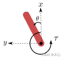
为了更好得观察到DQN存在的Q值估计overestimation的问题，我们使用gym中的Pendulum-v1的环境（详见官网），注意这里gym的版本为v26，

倒立摆的数据标注如下所示

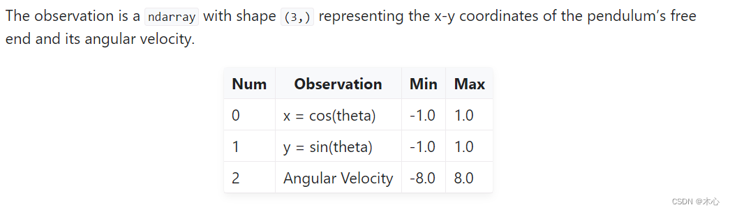
2.1 Obseravtion Space

2.2 Reward Function

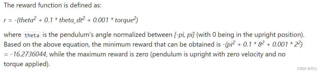
该环境的奖励函数为
$$-({\theta }^2+0.1{\dot{\theta }}^2+0.001a^2)$$
倒立摆向上保持不动的时候奖励为0，其余位置倒立摆的奖励为负数，所以该环境下动作值Q不会超过0。

2.3 Action Space

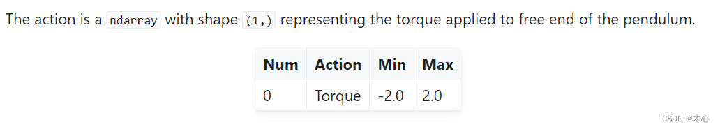
动作空间是一个连续值，是作用于倒立摆末端的扭矩。但是DQNs只能用于处理离散动作空间环境，因此我们无法直接使用DQNs来处理倒立摆环境，但是倒立摆环境会比较方便地验证Vanilla DQN存在对Q值过估计的问题。为了使得DQNs能够处理这种连续动作空间的环境，我们可以使用将连续动作空间离散化的方法，来达到伪连续的效果。

import gym
env_name = 'Pendulum-v1'
env = gym.make(id=env_name)
print("The minimum of action space is ", env.action_space.low[0])
print("The maximum of action space is ", env.action_space.high[0])def dis2con(discrete_action, action_dim, env):action_upbound = env.action_space.high[0]action_lowbound = env.action_space.low[0]return action_lowbound + discrete_action * (action_upbound - action_lowbound) / (action_dim - 1)# 示例将[-2.0,2.0]的连续动作空间转换成30维度离散动作空间
action_dim = 30 
discrete_action =  list(range(action_dim))
continue_action = []
for da in discrete_action:continue_action.append(dis2con(da, action_dim, env))
print(discrete_action)
print(continue_action)
env.close()

结果如下

The minimum of action space is  -2.0
The maximum of action space is  2.0
[0, 1, 2, 3, 4, 5, 6, 7, 8, 9, 10, 11, 12, 13, 14, 15, 16, 17, 18, 19, 20, 21, 22, 23, 24, 25, 26, 27, 28, 29]
[-2.0, -1.8620689655172413, -1.7241379310344827, -1.5862068965517242, -1.4482758620689655, -1.3103448275862069, -1.1724137931034484, -1.0344827586206895, -0.896551724137931, -0.7586206896551724, -0.6206896551724137, -0.48275862068965525, -0.3448275862068966, -0.2068965517241379, -0.06896551724137923, 0.06896551724137945, 0.2068965517241379, 0.34482758620689635, 0.48275862068965525, 0.6206896551724137, 0.7586206896551726, 0.896551724137931, 1.0344827586206895, 1.1724137931034484, 1.3103448275862069, 1.4482758620689653, 1.5862068965517242, 1.7241379310344827, 1.8620689655172415, 2.0]

3. DQNs Code

在本节，我们正式实现Vanilla DQN，Double DQN以及Dueling DQN并且观察对比其效果

import random
import collections
import torch
import torch.nn.functional as F
import numpy as np
from tqdm import tqdm
import gym
import matplotlib.pyplot as plt# Experience Replay
class ReplayBuffer():def __init__(self,  capacity):self.buffer = collections.deque(maxlen=capacity)def size(self):return len(self.buffer)def add(self, state, action, reward, next_state, done):self.buffer.append((state, action, reward, next_state, done))def sample(self, batch_size):transition = random.sample(self.buffer, batch_size)states, actions, rewards, next_states, dones = zip(*transition)return np.array(states), np.array(actions), np.array(rewards),  np.array(next_states), np.array(dones)# Value Approximation Net
class QNet(torch.nn.Module):# DDQN & VanillaDQN网络框架def __init__(self, state_dim, hidden_dim, action_dim):super(QNet,self).__init__()self.fc1 = torch.nn.Linear(state_dim, hidden_dim)self.fc2 = torch.nn.Linear(hidden_dim, action_dim)def forward(self,observation):x = F.relu(self.fc1(observation))x = self.fc2(x)return x# Advantage Net
class AVNet(torch.nn.Module):# DuelingDQN网络框架def __init__(self, state_dim, hidden_dim, action_dim):super(AVNet, self).__init__()self.fc1 = torch.nn.Linear(state_dim, hidden_dim)self.fc_V = torch.nn.Linear(hidden_dim, 1)self.fc_A = torch.nn.Linear(hidden_dim, action_dim)def forward(self, observation):x = F.relu(self.fc1(observation))V = self.fc_V(x)A = self.fc_A(x)Q = A + V - A.mean(dim=1).view(-1,1)return Q# Vanilla DQN algorithm & Double DNQ & Dueling DQN 
class DQNs():def __init__(self, state_dim, hidden_dim, action_dim, learning_rate, gamma, epsilon, target_update, device, dqn_type):self.action_dim = action_dimif dqn_type == "VanillaDQN" or dqn_type == "DoubleDQN":self.q_net = QNet(state_dim , hidden_dim, action_dim).to(device) # behavior net将计算转移到cuda上self.target_q_net = QNet(state_dim, hidden_dim, action_dim).to(device) # target netprint(self.q_net)elif dqn_type == "DuelingDQN": # DuelingDQN采取不同的网络框架self.q_net = AVNet(state_dim, hidden_dim, action_dim).to(device)self.target_q_net = AVNet(state_dim, hidden_dim, action_dim).to(device)self.optimizer = torch.optim.Adam(self.q_net.parameters(), lr=learning_rate)self.target_update = target_update  # 目标网络更新频率 self.gamma = gamma  # 折扣因子self.epsilon = epsilon # epsilon-greedyself.count = 0 # record update timesself.device = device # deviceself.dqn_type = dqn_type # VanillaDQN or DoubleDQN or DuelingDQNdef choose_action(self, state): # epsilon-greedy# one state is a list [x1, x2, x3, x4] if np.random.random() < self.epsilon:action = np.random.randint(self.action_dim) # 产生[0,action_dim)的随机数作为actionelse:state = torch.tensor([state], dtype=torch.float).to(self.device)action = self.q_net(state).argmax(dim=1).item()return actiondef max_q_values(self, state):state = torch.tensor([state], dtype=torch.float).to(self.device)return self.q_net(state).max(dim=1)[0].item()def learn(self, transition_dict):states = torch.tensor(transition_dict['states'], dtype=torch.float).to(self.device)next_states = torch.tensor(transition_dict['next_states'], dtype=torch.float).to(self.device)actions = torch.tensor(transition_dict['actions'], dtype=torch.int64).view(-1,1).to(self.device)rewards = torch.tensor(transition_dict['rewards'], dtype=torch.float).view(-1,1).to(self.device)dones = torch.tensor(transition_dict['dones'], dtype=torch.float).view(-1,1).to(self.device)q_values = self.q_net(states).gather(dim=1, index=actions)if self.dqn_type == 'DoubleDQN':    # DoubleDQNmax_action = self.q_net(next_states).max(dim=1)[1].view(-1,1)max_next_q_values = self.target_q_net(next_states).gather(dim=1, index=max_action)elif self.dqn_type == 'VanillaDQN' or dqn_type == 'DuelingDQN': # VanillaDQN & DuelingDQNmax_next_q_values = self.target_q_net(next_states).max(dim=1)[0].view(-1,1)q_target = rewards + self.gamma * max_next_q_values * (1 - dones)   # TD targetdqn_loss = torch.mean(F.mse_loss(q_target, q_values)) # 均方误差损失函数self.optimizer.zero_grad()dqn_loss.backward()self.optimizer.step()# 一定周期后更新target network参数if self.count % self.target_update == 0:self.target_q_net.load_state_dict(self.q_net.state_dict())self.count += 1def dis_to_con(discrete_action, env, action_dim):  # 离散动作转回连续的函数action_lowbound = env.action_space.low[0]  # 连续动作的最小值action_upbound = env.action_space.high[0]  # 连续动作的最大值return action_lowbound + (discrete_action /(action_dim - 1)) * (action_upbound -action_lowbound)# train DQN agent
def train_DQN_agent(env, agent, replaybuffer, num_episodes, batch_size, minimal_size, seed):return_list = []max_q_value = 0max_q_value_list = []for i in range(10):with tqdm(total=int(num_episodes/10), desc="Iteration %d"%(i+1)) as pbar:for i_episode in range(int(num_episodes/10)):episode_return = 0observation, _ = env.reset(seed=seed)done = Falsewhile not done:env.render()action = agent.choose_action(observation)max_q_value = agent.max_q_values(observation) * 0.005 + max_q_value * 0.995 # smooth the maximum q-valuemax_q_value_list.append(max_q_value)  # save maximum q-value# convert discrete action to pesudo-continuousaction_continuous = dis_to_con(action, env,agent.action_dim)observation_, reward, terminated, truncated, _ = env.step([action_continuous])done = terminated or truncatedreplaybuffer.add(observation, action, reward, observation_, done)observation = observation_episode_return += rewardif replaybuffer.size() > minimal_size:b_s, b_a, b_r, b_ns, b_d = replaybuffer.sample(batch_size)transition_dict  = {'states': b_s,'actions': b_a,'rewards': b_r,'next_states': b_ns,'dones': b_d}# print('\n--------------------------------\n')# print(transition_dict)# print('\n--------------------------------\n')agent.learn(transition_dict)return_list.append(episode_return)if (i_episode + 1) % 10 == 0:pbar.set_postfix({'episode':'%d' % (num_episodes / 10 * i + i_episode + 1),'return':'%.3f' % np.mean(return_list[-10:])})pbar.update(1)env.close()return return_list, max_q_value_list        def plot_curve(return_list, mv_return, algorithm_name, env_name):episodes_list = list(range(len(return_list)))plt.plot(episodes_list, return_list, c='gray', alpha=0.6)plt.plot(episodes_list, mv_return)plt.xlabel('Episodes')plt.ylabel('Returns')plt.title('{} on {}'.format(algorithm_name, env_name))plt.show()def moving_average(a, window_size):cumulative_sum = np.cumsum(np.insert(a, 0, 0)) middle = (cumulative_sum[window_size:] - cumulative_sum[:-window_size]) / window_sizer = np.arange(1, window_size-1, 2)begin = np.cumsum(a[:window_size-1])[::2] / rend = (np.cumsum(a[:-window_size:-1])[::2] / r)[::-1]return np.concatenate((begin, middle, end))if __name__ == "__main__":# reproducibleseed_number = 0random.seed(seed_number)np.random.seed(seed_number)torch.manual_seed(seed_number)# render or notrender = Falseenv_name = 'Pendulum-v1'hidden_dim = 128 # number of hidden layerslr = 2e-3   # learning ratenum_episodes = 500  # episode lengthgamma = 0.98 # discounted rateepsilon = 0.01 # epsilon-greedytarget_update = 10 # per step to update target networkbuffer_size = 10000 # maximum size of replay bufferminimal_size = 500 # minimum size of replay buffer to begin learningbatch_size = 64 # batch_size using to train the neural networkdevice = torch.device('cuda' if torch.cuda.is_available() else 'cpu')if render:  env = gym.make(id=env_name, render_mode='human')else:env = gym.make(id=env_name)state_dim = env.observation_space.shape[0]action_dim = 30 # discrete the action space to 30 dimensiondqn_type = 'DuelingDQN'  # VanillaDQN & DoubleDQN & DuelingDQNagent = DQNs(state_dim, hidden_dim, action_dim, lr, gamma, epsilon, target_update, device, dqn_type)replaybuffer = ReplayBuffer(buffer_size)return_list, max_q_value_list = train_DQN_agent(env, agent, replaybuffer, num_episodes, batch_size, minimal_size, seed_number)# plot moving average return curvemv_return = moving_average(return_list, 9)plot_curve(return_list, mv_return, dqn_type, env_name)# plot maximum q-value curveframe_list = list(range(len(max_q_value_list)))plt.plot(frame_list, max_q_value_list)plt.axhline(0, c='green', ls='--')plt.axhline(10, c='red', ls='--')plt.xlabel('Frames')plt.ylabel('Max Q Values')plt.title("{} on {}".format(dqn_type, env_name))plt.show()

3.1 Vanilla DQN效果

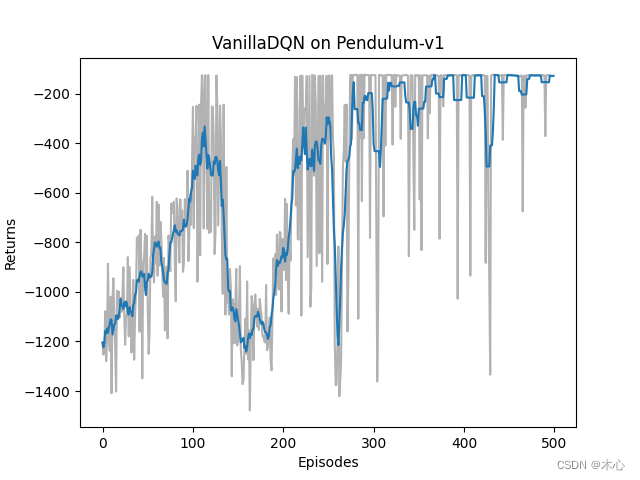
Vanilla DQN的学习回报（return）如下图

Vanilla DQN的最大Q值估计如图

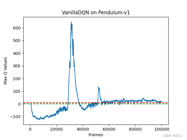
按照agent交互环境的分析，我们对Q值的估计不应该超过0，但是Vanilla DQN已经超过了600，这是很严重的过高估计的问题。

3.2 Double DQN效果

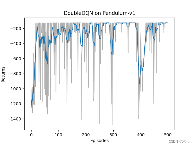
Double DQN的学习回报如下图

Double DQN的最大Q值估计如下图

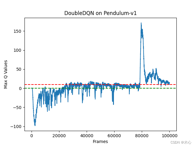
可以看出来Double DQN确实有效缓解了对最大Q值估计过高的问题。

3.3 Dueling DQN效果

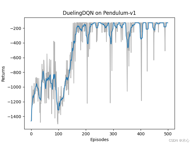
Dueling DQN的学习回报如下图

Dueling DQN的最大Q值估计如下图

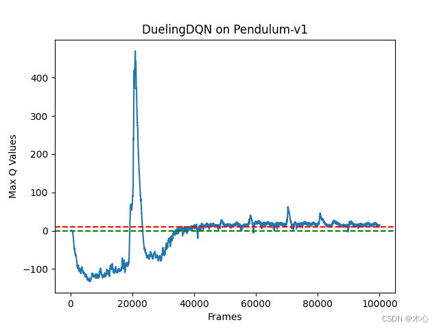
可以看出来Dueling DQN也能缓解对最大Q值估计过高的问题。

Reference

Materials
DQN及其多种变式
Hands on RL
Deep Reinforcement Learning with Double Q-learning
Reinforcement Learning with Code 【Code 1. Tabular Q-learning】
Reinforcement Learning with Code 【Chapter 7. Temporal-Difference Learning】
Reinforcement Learning with Code 【Code 4. Vanilla DQN】

Papers

• Vallina DQN

  Playing Atari with Deep Reinforcement Learning

• Double DQN

  Deep Reinforcement Learning with Double Q-learning

• Dueling DQN

  Dueling Network Architectures for Deep Reinforcement Learning